Accelerating Spectroscopic Data Processing Using Python and GPUs on NERSC Supercomputers
←
→
Page content transcription
If your browser does not render page correctly, please read the page content below
PROC. OF THE 20th PYTHON IN SCIENCE CONF. (SCIPY 2021)                                                                                                   33

    Accelerating Spectroscopic Data Processing Using
     Python and GPUs on NERSC Supercomputers
                                 Daniel Margala‡∗ , Laurie Stephey‡ , Rollin Thomas‡ , Stephen Bailey§

                                                                                  F

Abstract—The Dark Energy Spectroscopic Instrument (DESI) will create the              targets per frame is computationally intensive and has been the
most detailed 3D map of the Universe to date by measuring redshifts in light          primary focus of optimization efforts for several years ([RTD+ 17],
spectra of over 30 million galaxies. The extraction of 1D spectra from 2D spec-       [STB19]). The DESI data processing pipeline is predominantly
trograph traces in the instrument output is one of the main computational bot-        implemented using the Python programming language. A strict
tlenecks of DESI data processing pipeline, which is predominantly implemented
                                                                                      requirement from the DESI data processing team is to keep the
in Python. The new Perlmutter supercomputer system at the National Energy
Scientific Research and Computing Center (NERSC) will feature over 6,000
                                                                                      code implementation in Python.
NVIDIA A100 GPUs across 1,500 nodes. The new heterogenous CPU-GPU                          The existing state of the art implementation utilizes a divide
computing capability at NERSC opens the door for improved performance for             and conquer framework to make spectro-perfectionism algorithm
science applications that are able to leverage the high-throughput computation        tractable on existing computing hardware, see Figure 1. The
enabled by GPUs. We have ported the DESI spectral extraction code to run on           code utilizes the Message Passing Interface (MPI) via mpi4py to
GPU devices to achieve a 20x improvement in per-node throughput compared              exploit both multi-core and multi-node parallelism ([DPS05]). The
to the current state of the art on the CPU-only Haswell partition of the Cori
                                                                                      application uses multidimensional array data structures provided
supercomputer system at NERSC.
                                                                                      by NumPy along with several linear algebra and special functions
Index Terms—Python, HPC, GPU, CUDA, MPI, CuPy, Numba, mpi4py, NumPy,                  from the NumPy and SciPy libraries ([HMvdW+ 20], [VGO+ 20]).
SciPy, Astronomy, Spectroscopy                                                        Several expensive kernels are implemented using Numba just-in-
                                                                                      time compilation ([LPS15]). All input and output files are stored
                                                                                      on disk using the FITS file format. The application is parallelized
Introduction                                                                          by dividing an image into thousands of small patches, performing
The Dark Energy Spectroscopic Instrument (DESI) experiment                            the extraction on each individual patch in parallel, and stitching
is a cosmological redshift survey. The survey will create the                         the result back together.
most detailed 3D map of the Universe to date, using position                               This has worked well for CPU-only computing architectures
and redshift information from over 30 million galaxies. During                        such as the Haswell (Intel Xeon Processor E5-2698 v3) and
operation, around 1000 CCD frames per night (30 per exposure)                         Knights Landing (Intel Xeon Phi Processor 7250) partitions on the
are read out from the instrument and transferred to NERSC for                         Cori1 supercomputer at NERSC. The new Perlmutter2 supercom-
processing and analysis. Each frame contains 500 2D spectrograph                      puter system at NERSC will have a partition of GPU accelerated
traces from galaxies, standard stars (for calibration), or just the                   nodes (AMD EPYC 7763, NVIDIA A100 GPU). The goal of
sky (for background subtraction). These traces must be extracted                      this work is to speed up the DESI experiment’s data processing
from the CCD frames taking into account optical effects from                          pipeline by porting the spectroscopic extraction step to run on the
the instrument, telescope, and the Earth’s atmosphere. Redshifts                      GPU partition of the Perlmutter supercomputer at NERSC.
are measured from the extracted The data is processed in near-                             In early 2020, the team began reimplementing the existing
real time in order to monitor survey progress and update the                          extraction code specter 3 by reconsidering the problem. The DESI
observing schedule for the following night. Periodically, a com-                      spectral extraction problem is fundamentally an image process-
plete reprocessing of all data observed to-date is performed and                      ing problem which historically have been well-suited to GPUs.
made available as data release to the collaboration and eventually                    However, in many places, the existing CPU version of the code
released to the public.                                                               used loops and branching logic rather than vector or matrix-
    The DESI spectral extraction code is an implementation of the                     based operations. We performed a significant refactor switching
spectro-perfectionism algorithm, described in [BS10]. The process                     key parts of the analysis to matrix-based operations which would
of extracting 1D spectra from 2D spectrograph traces for all 500                      be well suited to massive GPU parallelism. Additionally, the
                                                                                      refactor enabled more flexible task partitioning and improved node
* Corresponding author: danielmargala@lbl.gov
‡ Lawrence Berkeley National Laboratory: National Energy Scientific Re-               utilization. From this refactor alone, still running only on the CPU,
search and Computing Center                                                           we obtained 1.6x speedup compared to the original CPU version.
§ Lawrence Berkeley National Laboratory: Physics Division
                                                                                      From here, we began our GPU implementation.
Copyright © 2021 Daniel Margala et al. This is an open-access article
distributed under the terms of the Creative Commons Attribution License,
which permits unrestricted use, distribution, and reproduction in any medium,           1. https://docs.nersc.gov/systems/cori/
provided the original author and source are credited.                                   2. https://docs.nersc.gov/systems/perlmutter/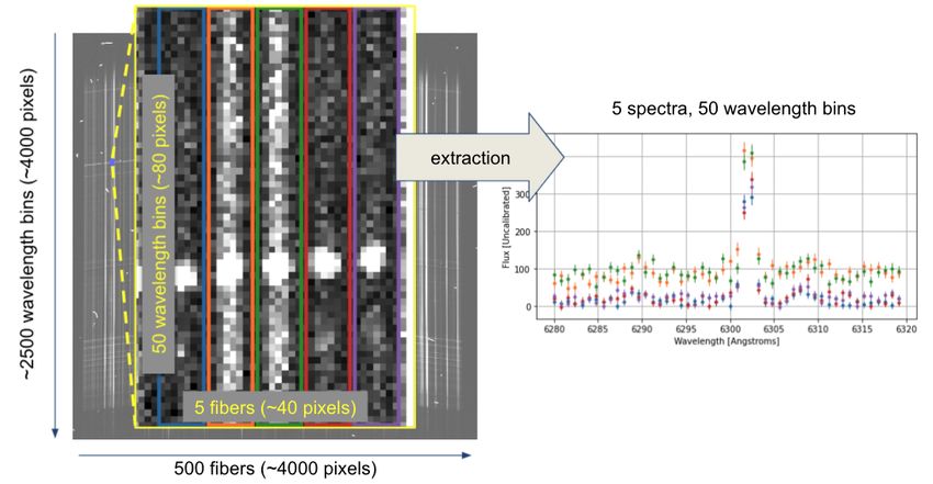
34 PROC. OF THE 20th PYTHON IN SCIENCE CONF. (SCIPY 2021)
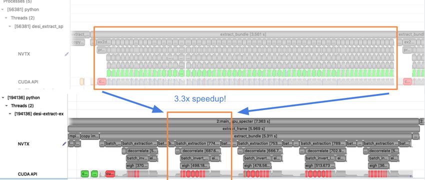
Fig. 1: The goal of the algorithm is to extract spectra from raw telescope output. Here we show the raw telescope output for a single "patch"
and the corresponding pieces of the extracted spectra. The divide and conquer strategy used in this application divides an image into roughly
5,000 patches which can be extracted in parallel. The extracted pieces are then stiched back together and written to disk for further processing
by the data pipeline.
We describe our iterative approach to porting and optimizing
the application using NVIDIA Nsight Systems for performance
analysis. We use a combination of CuPy and JIT-compiled CUDA
kernels via Numba for GPU-acceleration. In order to maximize
use of resources (both CPUs and GPUs), we use MPI via mpi4py
and CUDA Multi-Process Service. We discuss the lessons we
learned during the course of this work that will help guide future
efforts of the team and inform other science teams looking to
leverage GPU-acceleration in their Python-based data processing
applications. We project that new extraction code gpu_specter 4
running on Perlmutter will achieve a 20x improvement in per-
node throughput compared to the current production throughput
on Cori Haswell.
GPU Implementation
The existing CPU implementation uses NumPy and SciPy (BLAS
and LAPACK) for linear algebra, numba just-in-time compilation
for specialized kernels, and mpi4py (MPI) for multi-core and
multi-node scaling. The code is parallelized to run on multiple
CPU cores and nodes using a Single Program Multiple Data
Fig. 2: An illustration of the program structure highlighting main MPI
(SPMD) programming pattern enabled by MPI through mpi4py. communication points. Flow runs from top to bottom.
The structure of the program is illustrated in Figure 2, which
highlights the main MPI communication points.
In order to leverage the compute capabilities of GPU devices
run on GPU hardware, such as CuPy, pyCUDA, pytorch, JAX, and
and adhere to the DESI Python requirement, we decided to
Numba CUDA. We chose to use CuPy [OUN+ 17] and Numba
use a GPU-accelerated Python library. The main considerations
CUDA based on our ability to easily integrate their API with our
for heterogeneous CPU-GPU computing are to minimize data
existing code.
movement between the CPU host and the GPU device and to feed
the GPU large chunks of data that can be processed in parallel. The initial GPU port was implemented by off-loading compute
Keeping those considerations in mind, we left rest of the GPU intensive steps of the extraction to the GPU using CuPy in
programming details to external libraries. There are many rapidly place of NumPy and SciPy. A few custom kernels were also
maturing Python libraries that allow users to write code that will re-implemented using Numba CUDA just-in-time compilation. In
many cases, we merely replaced an existing API call from numpy,
3. https://github.com/desihub/specter scipy, or numba.jit with equivalent GPU-accelerated version from
4. https://github.com/desihub/gpu_specter cupy, cupyx.scipy, or numba.cuda.jit.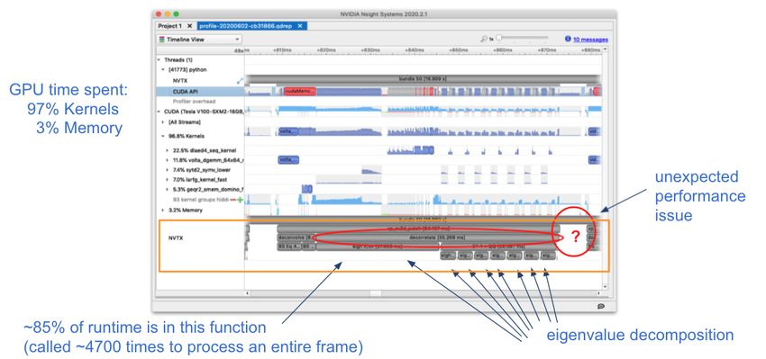
ACCELERATING SPECTROSCOPIC DATA PROCESSING USING PYTHON AND GPUS ON NERSC SUPERCOMPUTERS                                                  35

   The example code below demonstrates how we integrated                    Nsight Systems provides a zoomable timeline view that allows
cupy, numba.cuda, and the NumPy API:                                    us to visualize the performance of our code. Using Nsight Sys-
import cupy                                                             tems, we can see the regions of our code that we marked with
import numba.cuda                                                       NVTX wrappers, as well as the lower level memory and kernel
import numpy                                                            operations. In Figure 3, we show a screenshot from an early profile
                                                                        of our GPU port using the NSight Systems GUI. At a high-level,
# CUDA kernel
@numba.cuda.jit                                                         we see that memory transfers and kernel executions, respectively,
def _cuda_addone(x):                                                    account for 3% and 97% of the time spent on GPU. From this
   i = numba.cuda.grid(1)                                               profile, we identified that approximately 85% of the runtime of
   if i < x.size:
      x[i] += 1                                                         the application is spent in the "decorrelate" step of the algorithm.
                                                                        We also discovered an unexpected performance issue near the
# convenience wrapper with thread/block configuration                   end patch extraction that we were able to solve using NumPy
def addone(x):                                                          advanced array indexing. The execution time of the decorrelate
   # threads per block
   tpb = 32                                                             method is dominated by the eigenvalue decomposition operations.
   # blocks per grid                                                    Profiling also helped identify unexpected performance issues in
   bpg = (x.size + (tpb - 1)) // tpb                                    code regions we did not expect.
   _cuda_addone[bpg, tpb](x)

# create array on device using cupy                                     Maximizing Node Utilization
x = cupy.zeros(1000)                                                    We use multiple GPUs in our application via MPI (mpi4py).
# pass cupy ndarray to numba.cuda kernel                                Since the CPU implementation is already using MPI, minimal
addone(x)
# Use numpy api with cupy ndarray                                       refactor was required. Each MPI rank is assigned to a sin-
total = numpy.sum(x)                                                    gle GPU. Mapping MPI ranks to GPUs can be handled using
                                                                        slurm options (--gpu-bind ), setting environment variables such
We found that this interopability gave us a lot of flexibility to       as CUDA_VISIBLE_DEVICES, or at runtime using the CuPy
experiment during development. This achieved our initial goal           API (cupy.cuda.Device.use() ). We oversubscribe ranks to GPUs
porting the application to run on GPU hardware.                         to saturate GPU utilization using CUDA Multi-Process Service
    In the following sub-sections, we will discuss the major            (MPS), which allows kernel and memcopy operations from dif-
development milestones that lead to the improved performance            ferent processes to overlap on the GPU. Some care must be
of the application on GPUs.                                             taken to avoid over allocating memory on each device. We use
                                                                        a shell script wrapper to ensure the CUDA MPS control daemon
Profiling the Code                                                      is started by a single process on each node process server before
As discussed in previous work [STB19], the team found a lot of          launching our application. At NERSC, we use the following script
value using profiling tools such as the cProfile Python module.         which references environment variables set by the slurm workload
In this work, we used NVIDIA’s NSight Systems to profile                manager.
the application, identify bottlenecks in performance, and focus         #!/bin/bash
optimization efforts. We added CUDA NVTX markers (using the             # Example mps-wrapper usage:
                                                                        # > srun -n 2 -c 1 mps-wrapper command arg1 ...
CuPy API) to label regions of our code using descriptions that we       export CUDA_MPS_PIPE_DIRECTORY=/tmp/nvidia-mps
would be able to easily identify in the profile viewer. Without these   export CUDA_MPS_LOG_DIRECTORY=/tmp/nvidia-log
labels, it sometimes difficult to decipher the names of low-level       # Launch MPS from a single rank per node
                                                                        if [ $SLURM_LOCALID -eq 0 ]; then
kernels that are called indirectly by our application. We generally        nvidia-cuda-mps-control -d
used a following command to generate profiles of our application:       fi
                                                                        # Wait for MPS to start
nsys profile --sample=none \
                                                                        sleep 5
             --trace=cuda,nvtx \
                                                                        # Run the command
             --stats=true \
                                                                        "$@"
              \
                                                                        # Quit MPS control daemon before exiting
              \
                                                                        if [ $SLURM_LOCALID -eq 0 ]; then
             app.py
                                                                           echo quit | nvidia-cuda-mps-control
                                                                        fi
The nsys profile launches and profiles our application. Usuaully,
we disable CPU sampling (--sample=none) and only trace CUDA             In Figure 4, we show how performance scales with the number
and NVTX APIs (--trace=cuda,nvtx) to limit noise in the profile         of GPUs used and the number of MPI ranks per GPU. The solid
output. When using MPI, we add the mpirun or equivalent (srun           colored lines indicate the improved performance as we increase the
on NERSC systems) executable with its arguments following the           number of GPU used. Different colors represent varying degrees of
arguments to the nsys profile segment of the command. Simi-             the number of MPI ranks per GPU. In this case, using 2 MPI ranks
larily, when using the CUDA Multi-Process Service, we include           per GPU seems to saturate performance and we observe a slight
a wrapper shell script that ensures the service is launches and         degradation in performance oversubscribing further. We reached
shutdowns from a single process per node. Finally, we specify           the GPU memory limit when attempting to go beyond 4 MPI
the executable we wish to profile along with its arguments. The         ranks per GPU. The measurements for the analysis shown here
--stats=true option generates a set of useful summary statistics        were performed on test node at NERSC using 4 NVIDIA V100
that is printed to stdout. For a more detailed look at runtime          GPUs. The Perlmutter system will use NVIDIA A100 (40GB)
performance, it is useful view the generated report file using the      GPUs which have more cores and significantly more memory than
NSight Systems GUI.                                                     the V100 (16GB) GPUs. A similar analysis showed that we could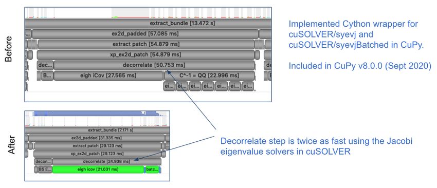
36                                                                                        PROC. OF THE 20th PYTHON IN SCIENCE CONF. (SCIPY 2021)

                          Fig. 3: A screenshot of a profile from an early GPU port using NVIDIA Nsight Systems.

go up to 5 MPI ranks per GPU on a test system with A100s. We           spectro-perfectionism algorithm, an eigenvalue decomposition is
note that while this configuration maximizes the expected GPU          performed on the inverse covariance matrix which is then used
utilization on a Perlmutter with 4 A100 GPUs, the 64-core AMD          to calculate the covariance matrix followed by several smaller
Milan CPU is only at 31.25% utilization with 20 MPI ranks. Later       eigenvalue decompositions that are performaned on the diagonal
on, we will discuss one way to utilize a few of these spare CPU        blocks of the covariance matrix. Since the small eigenvalue de-
cores.                                                                 compositions are performed on independent sub-matrices, we tried
                                                                       "batching" (or "stacking") the operations. We noted the existance
                                                                       of a syevjBatched function in CUDA cuSOLVER library which
                                                                       could perform eigenvalue decomposition on batches of input ma-
                                                                       trices using a Jacobi eigenvalue solver. This was not immediately
                                                                       available in Python via CuPy but we were able to implement
                                                                       Cython wrappers in CuPy using similar wrappers already present
                                                                       in CuPy as a guide. We submitted our implementation as a pull-
                                                                       request to the CuPy project on GitHub5 .
                                                                           In Figure 5, we show profile snippets of that demonstate the
                                                                       improved performance using the Jacobi eigenvalue solvers from
                                                                       the cuSOLVER library. The execution time of the "decorrelate"
                                                                       method improved by a factor of two.
                                                                           This inspired us to look for opportunities to use batched
                                                                       operations in our program. We found a significant speedup by
                                                                       refactoring the application to extract spectra from multiple patches
                                                                       in a subbundle using batched array and linear algebra operations.
                                                                       This allowed us to leverage batched Cholesky decomposition and
                                                                       solver operations on the GPU (potrfBatched and potrsBatched in
                                                                       the cuSOLVER library). We contributed cupyx.linalg.posv (named
                                                                       after LAPACK’s xPOSV routines) to solve the linear equations
                                                                       A x = b via Cholesky factorization of A, where A is a real
Fig. 4: Performance scaling with multiple NVIDIA V100 GPUs. The        symmetric or complex Hermitian positive-definite matrix6 . Our
solid colored lines indicate the improved performance as we increase   implementation was essentially a generalization of an existing
the number of GPU used. Different colors represent varying degrees
of the number of MPI ranks per GPU as indicated in the legend.
                                                                       method cupyx.linalg.invh, which was implemented as the special
The horizontal blue lines representing CPU-only measurements were      case where the right-hand side of the equation is the Identity
approximate and only used for reference.                               matrix. In Figure 6, we compare the profile timelines before
                                                                       and after implementing batch Cholesky decomposition and solver
                                                                       operations. The runtime for extraction over an entire subbundle of
Batching GPU Operations
                                                                       5 spectra is 3.3 times faster using batched Cholesky operations.

Earlier, we observed that eigenvalue decomposition accounted for         5. https://github.com/cupy/cupy/pull/3488
a significant portion of the execution time of our program. In the       6. https://github.com/cupy/cupy/pull/4291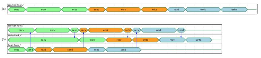
ACCELERATING SPECTROSCOPIC DATA PROCESSING USING PYTHON AND GPUS ON NERSC SUPERCOMPUTERS                                              37

                Fig. 5: The "decorrelate" is twice as fast using the Jacobi eigenvalue solvers from the cuSOLVER library.

                                    Fig. 6: Profile demonstrating speedup from batch Cholesky solve.

Overlapping Compute and IO                                            communicate to achieve this functionality. At a high level, the
                                                                      processing of a single frame can be broken down into 3 distinct
At this point, we observed that reading the input data and writing    phases: read, work, and write. The frames are processed in series,
the output results accounted for approximately 25%-30% of the         frame one (green) is processed, then frame two (orange), and
total wall time to process 30 frames from a single exposure in        finally frame (three). Panel a shows the non-overlapping sequence
series using a single node. The input data is read by a single MPI    of steps to process 3 frames in series. Panel b shows how the
rank, transferred to GPU memory, and then broadcast to other          overlapping of IO and computation is orchestrated using two
MPI ranks using CUDA-aware MPI. After extraction, each MPI            additional MPI ranks, dedicated reader and writer ranks. At the
rank transfers its results back to CPU memory and the results         start of the program, the reader rank reads the input data while
are gathered to the root MPI rank. The root MPI rank combines         all worker ranks wait. The reader rank performs some initial
the results and writes the output to a FITS file on disk. Using       preprocessing and sends the data to the root computation rank.
spare CPU cores, we were able to hide most of this IO latency         Once the data has been sent, the reader rank begins reading
and better utilize the resources available on a node. When there      the next frame. After the worker root receives the input data, it
are multiple frames processed per node, the write and read steps      performs the work which can involve broadcasting the data to
between successive frames can be interleaved with computation.        additional worker ranks in the computation group (not shown in
    In Figure 7, we demonstrate how a subset of the MPI ranks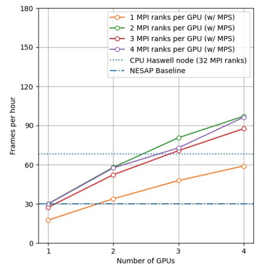
38                                                                                                   PROC. OF THE 20th PYTHON IN SCIENCE CONF. (SCIPY 2021)

the diagram). The result on the root computation rank is then sent                Numpy-compatible and SciPy-compataible APIs and, of course,
to a specially designated writer rank. The computation group ranks                the excellent foundation provided by NumPy and SciPy projects.
move on to processing the next frame which has already been read                  Profiling tools such as NVIDA Nsight Systems and the cProfile
from disk by a specially designated read rank. Meanwhile, the                     Python module often provide actionable insights to that can focus
writer rank finishes writing the previous result and is now waiting               optimization efforts. Refactoring code to expose parallelism and
to receive the next result.                                                       use more vectorized operations often improves performance on
    Overlapping compute and IO in this manner effectively hides                   both CPU and GPU computing architectures. For DESI, the
the intermediate read and write operations between frames pro-                    transition to GPUs on Perlmutter will shorten the time it takes
cessed serially on a node, reducing the wall time by over 60                      to process years worth of data from weeks to months down to
seconds and providing a 1.34x speedup in per-node throughput.                     hours to days.

Results
                                                                                  Acknowledgements
Throughout development, we performed a standard benchmark
after major feature implementations to track progress over time.                  This research used resources of the National Energy Research
For DESI, a useful and practical benchmark of performance is                      Scientific Computing Center (NERSC), a U.S. Department of
the number of frames that can be processed per node-time on                       Energy Office of Science User Facility located at Lawrence
NERSC systems. Specifically, we use the throughput measure                        Berkeley National Laboratory, operated under Contract No. DE-
frames-per-node-hour (FPNH) as the figure of merit (FoM) for                      AC02-05CH11231.
this application. This figure enables DESI to cost out how much                       This research is supported by the Director, Office of Sci-
data it can process given a fixed allocation of compute resources.                ence, Office of High Energy Physics of the U.S. Department
    A summary of benchmark results by major feature milestone                     of Energy under Contract No. DE–AC02–05CH11231, and by
is shown in Figure 8 and listed in Table 1. The benchmark uses                    the National Energy Research Scientific Computing Center, a
data from a single exposure containing 30 CCD frames. After                       DOE Office of Science User Facility under the same contract;
major feature implementations, we typically perform a scan of hy-                 additional support for DESI is provided by the U.S. National
perparameter values to identify the optimal settings. For example,                Science Foundation, Division of Astronomical Sciences under
after the "batch-subbundle" implementation, the optimal number                    Contract No. AST-0950945 to the NSF’s National Optical-Infrared
of wavelength bins per patch changed from 50 to 30. The baseline                  Astronomy Research Laboratory; the Science and Technologies
FoM for this application on the Edison and Cori supercomputers                    Facilities Council of the United Kingdom; the Gordon and Betty
is 27.89 FPNH and 40.15 FPNH, respectively. The initial refactor                  Moore Foundation; the Heising-Simons Foundation; the French
improved the CPU-only performance on Cori Haswell by more                         Alternative Energies and Atomic Energy Commission (CEA);
than 50%. Our initial GPU port achieved 6.15 FPNH on Cori                         the National Council of Science and Technology of Mexico;
GPU nodes, an unimpressive mark compared to the baseline CPU                      the Ministry of Economy of Spain, and by the DESI Member
benchmarks. Using visual profiling to guide optimization effort,                  Institutions. The authors are honored to be permitted to conduct
we were able to iterively improve the performance to 362.2 FPNH                   astronomical research on Iolkam Du’ag (Kitt Peak), a mountain
on Cori GPU nodes.                                                                with particular significance to the Tohono O’odham Nation.
    Since the Perlmutter system is not available at the time of
writing, we estimate the expected performance by running the
benchmark on an NVIDIA DGX-A100 system. A Perlmutter GPU
node will have the same NVIDIA A100 GPUs as the DGX system                        R EFERENCES
and the newer AMD Milan CPU compared to the AMD Rome
                                                                                  [BS10]      Adam S. Bolton and David J. Schlegel. Spectro-Perfectionism:
CPU on DGX. The projected FoM for this application on the                                     An Algorithmic Framework for Photon Noise-Limited Ex-
new Perlmutter supercomputer is 575.25 FPNH, a roughly 20x                                    traction of Optical Fiber Spectroscopy. Publications of the
improvement over the Edison baseline.                                                         Astronomical Society of the Pacific, 122(888):248, February
    Going forward, the team will need to re-evaluate where to                                 2010. doi:10.1086/651008.
                                                                                  [DPS05]     Lisandro Dalcín, Rodrigo Paz, and Mario Storti. MPI for
refocus optimization efforts. The performance of the spectral                                 Python. Journal of Parallel and Distributed Computing,
extraction step is now comparable to other steps in the DESI data                             65(9):1108–1115, 2005. doi:10.1016/j.jpdc.2005.
processing pipeline. We are currently evaluating other steps in the                           03.010.
DESI pipeline for GPU acceleration. The DESI team may also                        [HMvdW+ 20] Charles R. Harris, K. Jarrod Millman, Stéfan J. van der
                                                                                              Walt, Ralf Gommers, Pauli Virtanen, David Cournapeau, Eric
opt to spend the improved efficiency to perform more compute                                  Wieser, Julian Taylor, Sebastian Berg, Nathaniel J. Smith,
intensive processing if there is a scientific opportunity.                                    Robert Kern, Matti Picus, Stephan Hoyer, Marten H. van
                                                                                              Kerkwijk, Matthew Brett, Allan Haldane, Jaime Fernández del
                                                                                              Río, Mark Wiebe, Pearu Peterson, Pierre Gérard-Marchant,
Conclusion                                                                                    Kevin Sheppard, Tyler Reddy, Warren Weckesser, Hameer
                                                                                              Abbasi, Christoph Gohlke, and Travis E. Oliphant. Array pro-
The rising popularity of heterogenous CPU-GPU computing plat-                                 gramming with NumPy. Nature, 585(7825):357–362, Septem-
forms offers an opportunity for improving the performance of                                  ber 2020. URL: https://doi.org/10.1038/s41586-020-2649-2,
science applications. Adapting scientific Python applications to                              doi:10.1038/s41586-020-2649-2.
use GPU devices is relatively seamless due to the community                       [LPS15]     Siu Kwan Lam, Antoine Pitrou, and Stanley Seibert. Numba:
                                                                                              A LLVM-Based Python JIT Compiler. In Proceedings of
of developers working on GPU-accelerated libraries that provide                               the Second Workshop on the LLVM Compiler Infrastructure
                                                                                              in HPC, LLVM ’15, New York, NY, USA, 2015. Associa-
   *. Note that the initial-gpu benchmark only processed a single frame instead               tion for Computing Machinery. URL: https://doi.org/10.1145/
of all 30 frames from an expoosure.                                                           2833157.2833162, doi:10.1145/2833157.2833162.
ACCELERATING SPECTROSCOPIC DATA PROCESSING USING PYTHON AND GPUS ON NERSC SUPERCOMPUTERS 39
Fig. 7: Overlapping IO and compute. In panel a, we show an example timeline of the root worker MPI rank performing the read, work, and
write steps to process 3 frames. In panel b, we show an example timeline of the root worker, read, and write MPI ranks performing the read,
work, and write steps along with their inter-communication to process 3 frames.
Note System Arch Nodes GPUs MPI Ranks Walltime FPNH
(CPU/GPU) Per Node Per Node (sec)
Edison Xeon 25 - 24 154.9 27.89
baseline
Cori Haswell 19 - 32 141.6 40.15
cpu-refactor Cori Haswell 2 - 32 830.2 65.05
initial-gpu CoriGPU Skylake/V100 1 1 1 585.5* 6.15
CoriGPU Skylake/V100 2 4 8 611.6 88.30
multi-gpu
DGX Rome/A100 2 4 16 526.8 102.51
CoriGPU Skylake/V100 2 4 8 463.7 116.46
batch-eigh
DGX Rome/A100 2 4 16 372.7 144.90
batch- CoriGPU Skylake/V100 1 4 8 458.9 235.36
subbundle DGX Rome/A100 1 4 20 252.4 427.86
CoriGPU Skylake/V100 1 4 10 362.2 298.19
interleave-io
DGX Rome/A100 1 4 22 187.7 575.25
TABLE 1: Summary of benchmark results by major feature milestone.
PyHPC’17, New York, NY, USA, 2017. Association for Com-
puting Machinery. doi:10.1145/3149869.3149873.
[STB19] Laurie A. Stephey, Rollin C. Thomas, and Stephen J. Bailey.
Optimizing Python-Based Spectroscopic Data Processing on
NERSC Supercomputers. In Chris Calloway, David Lippa,
Dillon Niederhut, and David Shupe, editors, Proceedings of
the 18th Python in Science Conference, pages 69 – 76, 2019.
doi:10.25080/Majora-7ddc1dd1-00a.
[VGO+ 20] Pauli Virtanen, Ralf Gommers, Travis E. Oliphant, Matt
Haberland, Tyler Reddy, David Cournapeau, Evgeni Burovski,
Pearu Peterson, Warren Weckesser, Jonathan Bright, Sté-
fan J. van der Walt, Matthew Brett, Joshua Wilson, K. Jar-
rod Millman, Nikolay Mayorov, Andrew R. J. Nelson, Eric
Jones, Robert Kern, Eric Larson, C J Carey, İlhan Polat,
Yu Feng, Eric W. Moore, Jake VanderPlas, Denis Laxalde,
Josef Perktold, Robert Cimrman, Ian Henriksen, E. A. Quin-
tero, Charles R. Harris, Anne M. Archibald, Antônio H.
Ribeiro, Fabian Pedregosa, Paul van Mulbregt, and SciPy
1.0 Contributors. SciPy 1.0: Fundamental Algorithms for
Scientific Computing in Python. Nature Methods, 17:261–272,
Fig. 8: DESI Figure-of-Merit progress by major feature milestone. 2020. doi:10.1038/s41592-019-0686-2.
[OUN+ 17] Ryosuke Okuta, Yuya Unno, Daisuke Nishino, Shohei Hido,
and Crissman Loomis. CuPy: A NumPy-Compatible Library
for NVIDIA GPU Calculations. In Proceedings of Workshop
on Machine Learning Systems (LearningSys) in The Thirty-
first Annual Conference on Neural Information Processing
Systems (NIPS), 2017. URL: http://learningsys.org/nips17/
assets/papers/paper_16.pdf.
[RTD+ 17] Zahra Ronaghi, Rollin Thomas, Jack Deslippe, Stephen Bailey,
Doga Gursoy, Theodore Kisner, Reijo Keskitalo, and Julian
Borrill. Python in the NERSC Exascale Science Applications
Program for Data. In Proceedings of the 7th Workshop
on Python for High-Performance and Scientific Computing,You can also read