Advanced Econometrics 2, Hilary term 2021 Deep Neural Nets - Maximilian Kasy
←
→
Page content transcription
If your browser does not render page correctly, please read the page content below
Neural Nets

              Advanced Econometrics 2, Hilary term 2021
                         Deep Neural Nets

                                 Maximilian Kasy

                       Department of Economics, Oxford University

                                                                    1 / 21
Neural Nets
Agenda
I What are neural nets?
I Network design:
I Activation functions,
I network architecture,
I output layers.
I Calculating gradients for optimization:
I Backpropagation,
I stochastic gradient descent.
I Regularization using early stopping.
2 / 21Neural Nets
Takeaways for this part of class
I Deep learning is regression with complicated functional forms.
I Design considerations in feedforward networks include depth, width, and the
connections between layers.
I Optimization is difficult in deep learning because of
1. lots of data
2. and even more parameters
3. in a highly non-linear model.
I ⇒ Specially developed optimization methods.
I Cross-validation for penalization is computationally costly, as well.
I A popular alternative is sample-splitting and early stopping.
3 / 21Neural Nets
Setup
Deep Neural Nets
Setup
I Deep learning is (regularized) maximum likelihood, for regressions with complicated
functional forms.
I We want, for instance, to find θ to minimize
E (Y − f (X , θ ))2
for continuous outcomes Y , or to maximize
" #
y
E ∑ 1(Y = y ) · f (X , θ )
y
for discrete outcomes Y .
4 / 21Neural Nets
Setup
What’s deep about that?
Feedforward nets
I Functions f used for deep (feedforward) nets can be written as
f (x , θ ) = f k (f k −1 (. . . f 1 (x , θ 1 ), θ 2 ), . . . , θ k ).
I Biological analogy:
I Each value of a component of f j corresponds to the “activation” of a “neuron.”
I Each f j corresponds to a layer of the net.
Many layers ⇒ “deep” neural net.
I The layer-structure and the parameters θ determine how these neurons are connected.
I Inspired by biology, but practice moved away from biological models.
I Best to think of as a class of nonlinear functions for regression.
5 / 21Neural Nets
Setup
So what’s new?
I Very non-linear functional forms f . Crucial when
I mapping pixel colors into an answer to “Is this a cat?,”
I or when mapping English sentences to Mandarin sentences.
I Probably less relevant when running Mincer-regressions.
I Often more parameters than observations.
I Not identified in the usual sense.
But we care about predictions, not parameters.
I Overparametrization helps optimization:
Less likely to get stuck in local minima.
I Lots of computational challenges.
1. Calculating gradients:
Backpropagation, stochastic gradient descent.
2. Searching for optima.
3. Tuning: Penalization, early stopping.
6 / 21Neural Nets
Network design
Network design
Activation functions
I Basic unit of a net: a neuron i in layer j.
I Receives input vector xij (output of other
neurons).
I Produces output g (xij θij + ηij ).
I Activation function g (·):
I Older nets: Sigmoid function
(biologically inspired).
I Modern nets: “Rectified linear units:”
g (z ) = max(0, z ).
More convenient for getting gradients.
7 / 21Neural Nets
Network design
Network design
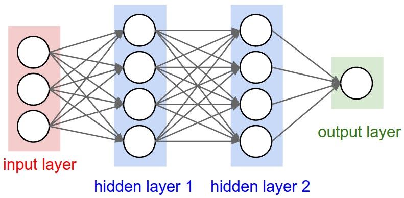
Architecture
I These neurons are connected, usually structured by layers.
Number of layers: Depth. Number of neurons in a layer: Width.
I Input layer: Regressors.
I Output layer: Outcome variables.
I A typical example:
8 / 21Neural Nets
Network design
Network design
Architecture
I Suppose each layer is fully connected to the next, and we are using RELU activation
functions.
I Then we can write in matrix notation (using componentwise max):
x j = f j (x j −1 , θ j ) = max(0, x j −1 · θ j + ηj )
I Matrix θ j :
I Number of rows: Width of layer j − 1.
I Number of columns: Width of layer j.
I Vector x j :
I Number of entries: Width of layer j.
I Vector ηj :
I Number of entries: Width of layer j.
I Intercepts. Confusingly called “bias” in machine learning.
9 / 21Neural Nets
Network design
Network design
Output layer
I Last layer is special: Maps into predictions.
I Leading cases:
1. Linear predictions for continuous outcome variables,
f k (x k −1 , θ k ) = x k −1 · θ k .
2. Multinomial logit (aka “softmax”) predictions for discrete variables,
exp(xjk −1 · θjk )
f kyj (x k −1 , θ k ) =
∑j 0 exp(xjk0 −1 · θjk0 )
I Network with only output layer: Just run OLS / multinomial logit.
10 / 21Neural Nets
Back propagation
The gradient of the likelihood
Practice problem
Consider a fully connected feedforward net with rectified linear unit activation functions.
1. Write out the derivative of its likelihood, for n observations, with respect to any
parameter.
2. Are there terms that show up repeatedly, for different parameters?
3. In what sequence would you calculate the derivatives,
in order to minimize repeat calculations?
4. Could you parallelize the calculation of derivatives?
11 / 21Neural Nets
Back propagation
Backpropagation
The chain rule
I In order to maximize the (penalized) likelihood, we need its gradient.
I Recall f (x , θ ) = f k (f k −1 (. . . f 1 (x , θ 1 ), θ 2 ), . . . , θ k ).
I By the chain rule:
0 0 0
!
∂ f (x , θ ) k
∂ f j (x j , θ j ) ∂ f j (x j −1 , θ j )
= ∏ 0 · .
∂ θij j 0 =j +1
∂ x j −1 ∂ θij
I A lot of the same terms show up in derivatives w.r.t different θij :
I x j 0 (values of layer j 0 ),
j0 j0 j0
I ∂ f (xj 0 −,θ1 ) (intermediate layer derivatives w.r.t. x j 0 −1 ).
∂x
12 / 21Neural Nets
Back propagation
Backpropagation
I Denote z j = x j −1 θ j + η j . Recall x j = max(0, z j ).
I Note ∂ x j /∂ z j = 1(z j ≥ 0) (componentwise), and ∂ z j /∂ θ j = x j −1
I First, forward propagation:
Calculate all the z j and x j , starting at j = 1.
I Then backpropagation:
Iterate backward, starting at j = k :
1. Calculate and store
∂ f (x , θ ) ∂ f (x , θ )
= · 1(z j ≥ 0) · θ j 0 .
∂ x j −1 ∂ xj
2. Calculate
∂ f (x , θ ) ∂ f (x , θ )
= · 1(z j ≥ 0) · x j −1 .
∂θj ∂ xj
13 / 21Neural Nets
Back propagation
Backpropagation
Advantages
I Backpropagation improves efficiency by storing intermediate derivatives, rather than
recomputing them.
I Number of computations grows only linearly in number of parameters.
I The algorithm is easily generalized to more complicated network architectures and
activation functions.
I Parallelizable across observations in the data (one gradient for each observation!).
14 / 21Neural Nets
Stochastic gradient descent
Stochastic gradient descent
I Gradient descent updates parameter estimates in the direction of steepest descent:
n
1
gt = ∑ ∇θ m(Xi , Yi , θ )
n i =1
θt +1 = θt − εt gt .
I Stochastic gradient descent (SGD) does the same, but instead uses just a random
subsample Bt = {i1t , . . . , ibt } (changing across t) of the data:
1
ĝt = ∑ ∇θ m(Xi , Yi , θ )
b i ∈Bt
θt +1 = θt − εt ĝt .
15 / 21Neural Nets
Stochastic gradient descent
Stochastic gradient descent
I We can do this because the full gradient is a sum of gradients for each observation.
I Typically, the batches Bt cycle through the full dataset.
I If the learning rate εt is chosen well, some convergence guarantees exist.
I The built-in randomness might help avoiding local minima.
I Extension: SGD with momentum,
vt = α vt −1 − εt ĝt ,
θt +1 = θt + vt .
I Initialization matters. Often start from previously trained networks.
16 / 21Neural Nets
Stochastic gradient descent
Why SGD makes sense
I The key observation that motivates SGD is that in an (i.i.d.) sampling context, further
observations become more and more redundant.
I Formally, the standard error of a gradient estimate based on b observations is of order
√
1/ b.
I But the computation time is of order b.
I Think of a very large data-set. Then it would take forever to just calculate one gradient,
and do one updating step.
I During the same time, SGD might have made many steps and come considerably
closer to the truth.
I Bottou et al. (2018) formalize these arguments.
17 / 21Neural Nets
Stochastic gradient descent
Excursion: Data vs. computation as binding constraint
I This is a good point to clarify some distinctions between the approaches of
statisticians and computer scientists.
I Consider a regularized m-estimation problem.
I Suppose you are constrained by
1. a finite data set,
2. a finite computational budget.
I Then the difference between any estimate and the estimand has three components:
1. Sampling error (variance),
2. approximation error (bias),
3. optimization error (failing to find the global optimum of your regularized objective
function).
18 / 21Neural Nets
Stochastic gradient descent
Statistics and computer science
I Statistical decision theory focuses on the trade-off between variance and bias.
I This makes sense if data-sets are small relative to computational capacity, so that
optimization error can be neglected.
I Theory in computer science often focuses on optimization error.
I This makes sense if data-sets are large relative to computational capacity, so that
sampling error can be neglected.
I Which results are relevant depends on context!
I More generally, I believe there is space for interesting theory that explicitly trades off all
three components of error.
19 / 21Neural Nets
Early stopping
Regularization for neural nets
I To get good predictive performance, neural nets need to be regularized.
I As before, this can be done using penalties such as λ kθ k22 (“Ridge”) or λ kθ k1
(“Lasso”).
I Problem: Tuning using cross-validation is often computationally too costly for deep
nets.
I An alternative regularization method is early stopping:
I Split the data into a training and a validation sample.
I Run gradient-based optimization method on the training sample.
I At each iteration, calculate prediction loss in the validation sample.
I Stop optimization algorithm when this prediction loss starts increasing.
20 / 21Neural Nets
References
References
I Goodfellow, I., Bengio, Y., and Courville, A. (2016). Deep learning. MIT Press,
chapters 6-8.
I Bottou, L., Curtis, F. E., and Nocedal, J. (2018). Optimization methods for large-
scale machine learning. SIAM Review, 60(2):223–311
21 / 21You can also read