An introduction to coupled ocean-atmosphere dynamics - Chris Roberts ECMWF Predictability Training Course, 23th March 2021

An introduction to coupled ocean-
atmosphere dynamics
Chris Roberts
Earth System Predictability Section, ECMWF
chris.roberts@ecmwf.int

ECMWF Predictability Training Course, 23th March 2021

 © ECMWF March 22, 2021

Topics covered in this lecture
• Why couple to a dynamic ocean?
 – Ocean coupling in the ECMWF Integrated Forecasting System (IFS)
 – Role of the oceans in Earth System Predictability
 – Timescales of ocean-atmosphere interaction

• Oceanography fundamentals
 – Features of the global ocean circulation
 – Governing equations and important balances

• Examples of air-sea interaction and its scale-dependence
 – Tropics vs mid-latitudes

• Challenges for coupled ocean-atmosphere forecasting
 – Horizontal resolution
 – Initializing the ocean state

 EUROPEAN CENTRE FOR MEDIUM-RANGE WEATHER FORECASTS October 29, 2014 2

Things that are not covered in this lecture
• Discussion of the MJO – see lecture by Frederic Vitart
• Detailed discussion of ENSO – see lecture by Magdalena Balmaseda

 EUROPEAN CENTRE FOR MEDIUM-RANGE WEATHER FORECASTS October 29, 2014 3

Why use a coupled model?

EUROPEAN CENTRE FOR MEDIUM-RANGE WEATHER FORECASTS October 29, 2014

The ECMWF Integrated Forecasting System (2020)

 Coupled IFS • All operational configurations of ECMWF IFS
 include dynamic representations of the ocean,
 Atmosphere (IFS cycle 46R1) atmosphere, sea ice, land surface, and ocean
 waves.
 Waves (ECWAM) Land (HTESSEL)
 • Sub-models exchange information hourly
 IFS to NEMO:
 • Radiation
 • Net precipitation
 • The IFS single-executable coupling strategy is
 NEMO to IFS:
 • SST
 • Wind stress described by Mogenson et al. (2012), EC Tech
 • Other terms for ice thermodyn.
 • Sea-ice concentration (+ other) Memo 673.
 • Surface currents
 • IFS cycles are documented on the ECMWF
Sea ice (LIM2) website: https://www.ecmwf.int/en/publications/ifs-
 Ocean (NEMO v3.4) documentation.
• Tripolar ORCA025 grid: ~0.25 degrees (~25 km)
• 75 vertical levels (~1m at surface) • An overview of the IFS coupled model is
• 20 minute time-step available in Roberts et al. (2018), Geoscientifc
 Model Development, 11, 3681-3712.

 EUROPEAN CENTRE FOR MEDIUM-RANGE WEATHER FORECASTS October 29, 2014 5

How does the ocean contribute to Earth System Predictability?
1) Coupling. Inclusion of a dynamic ocean allows ocean-atmosphere feedbacks.

 • Case study of tropical cyclone
 Neoguri (2014).

 • 5-day SST forecasts
 with/without ocean coupling.

 • Inclusion of a dynamic ocean
 allows simulation of a strong
 cold wake, which in turn
 impacts the evolution of the
 overlying cyclone.

 EUROPEAN CENTRE FOR MEDIUM-RANGE WEATHER FORECASTS October 29, 2014 6

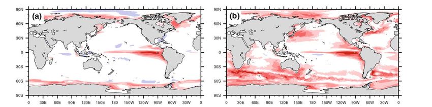
How does the ocean contribute to Earth System Predictability?
2) Persistence. Relative to the atmosphere, the ocean has a large heat capacity and much slower
adjustment time-scales (i.e. the ocean has a longer “memory”).

 Week 4 anomaly correlation for near- Week 4 anomaly correlation for sea
 surface (2m) atmospheric temperature. surface height (largely determined by
 ocean heat content).

 EUROPEAN CENTRE FOR MEDIUM-RANGE WEATHER FORECASTS October 29, 2014 7

How does the ocean contribute to Earth System Predictability?
3) Predictable ocean dynamics.
 Predictable ocean dynamics play an important role in
 modes of coupled ocean-atmosphere variability (e.g.
 ENSO).

 This example shows an idealized model (linear shallow-
 water dynamics) response to a westerly wind stress
 anomaly associated with El Nino conditions:
 - eastward-moving downwelling Kelvin wave.
 - upwelling Rossby waves propagating westward.

 Rossby waves reflect off the western boundary and
 propagate eastward as upwelling Kelvin waves, which
 raise thermocline and acts to reduce initial SST
 warming. See “delayed oscillator theory” (Battisti and
 Hirst, 1989; Suarez and Schopf, 1988).

 This type of large-scale equatorial wave dynamics is
 Image credit: Introduction to Tropical Meteorology, 2nd Edition. well-resolved by global ocean models.
 EUROPEAN CENTRE FOR MEDIUM-RANGE WEATHER FORECASTS October 29, 2014

Timescales of ocean-atmosphere interaction
 Climate change

 Climate variability

 Weather

Hours Days Weeks Months Years Decades Centuries
 Equatorial wave dynamics Mid-latitude Rossby waves Ocean heat
Diurnal cycle (SSTs Madden-Julian
and interaction with Oscillation (MJO) uptake (SLR)
 Gyre dynamics
 convection)
 El Nino-Southern Oscillation (ENSO) Atlantic multidecadal variability (AMV)
 Tropical cyclones
 Surface Indian Ocean Dipole (IOD) Pacific Decadal Oscillation (PDO)
 Tropical instability
 waves
 waves
 Seasonal mixed layer – Atlantic meridional overturning circulation (AMOC) variability
 Medium-range “reemergence”

 Extended-range

 Seasonal

 Ocean and atmosphere reanalyses
 EUROPEAN CENTRE FOR MEDIUM-RANGE WEATHER FORECASTS October 29, 2014

Oceanography fundamentals (1):
Features of the global ocean circulation

EUROPEAN CENTRE FOR MEDIUM-RANGE WEATHER FORECASTS October 29, 2014

Ocean vs atmosphere
Oceans have boundaries!

The heat capacity of the ocean is ~1000 times larger than that of the atmosphere.

The (incompressible) ocean is strongly stratified in the vertical with less dense (warmer and/or
fresher) layers at the surface. Deep convection is limited to the high latitudes.

In the ocean, dynamic (momentum) and thermodynamic (heat, freshwater) forcings are
concentrated at the surface. In the atmosphere, diabatic processes are important (i.e. there is
condensation) and radiation can interact with the entire atmospheric column.

The main challenge in ocean modelling is representation of small scale dynamical processes.

The main challenge in atmospheric modelling (or one of them) is the representation of the complex
coupling between dynamic and thermodynamic processes (e.g. interactions between the resolved
flow, clouds, convection, and radiative processes).

 EUROPEAN CENTRE FOR MEDIUM-RANGE WEATHER FORECASTS October 29, 2014 11

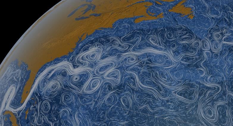
The wind-driven ocean circulation

 Image credit: Ocean Circulation 2nd Edition, The Open University

The horizontal ocean circulation is largely wind driven. It is characterized by large-scale sub-tropical and sub-polar
gyres, intense western boundary currents, coastal upwelling, strong equatorial currents, and the Antarctic Circumpolar
Current.

 EUROPEAN CENTRE FOR MEDIUM-RANGE WEATHER FORECASTS October 29, 2014

Thermohaline and overturning circulations
• The thermohaline circulation (THC) is associated with large scale (vertical) overturning circulations and is driven by fluxes
 of heat and fresh water.

• The Atlantic component of the THC is often referred to as the Atlantic Meridional Overturning Circulation (AMOC).

 EUROPEAN CENTRE FOR MEDIUM-RANGE WEATHER FORECASTS October 29, 2014

Ocean heat transports
• Overturning circulations play a particularly important role in meridional ocean heat transports: warm water
 transported polewards in upper layers is balanced by cold water transported equatorward in deeper layers.

• In the Atlantic, the northward heat transport by the vertical overturning circulation is much larger than that by the
 horizontal gyre circulation.

 Estimates of the globally integrated northward heat transport Atlantic ocean heat transports at 26N
 Total
 Ocean
 Atmosphere

 Image credit: Trenberth and Caron (2001)

 EUROPEAN CENTRE FOR MEDIUM-RANGE WEATHER FORECASTS October 29, 2014
 Image credit: Johns et al. (2011)

Oceanography fundamentals (2):
Governing equations and important properties

 EUROPEAN CENTRE FOR MEDIUM-RANGE WEATHER FORECASTS October 29, 2014

Governing equations for the ocean (+ typical approximations)

 advection (non-linear) pressure gradient

 Momentum
 conservation
 (F=ma)

tendency rotation/Coriolis frictional/viscous

 Vertical momentum equation (hydrostatic approximation)

 Mass conservation (incompressible, Boussinesq approx)

 Heat/salt conservation and
 equation of state for seawater

 EUROPEAN CENTRE FOR MEDIUM-RANGE WEATHER FORECASTS October 29, 2014

Dimensional analysis Typical values for basin-scale flow
Zonal momentum (neglect frictional/viscous terms for now)

Zonal momentum (dimensionless)

 Dimensionless variables

 Dominant balance is between pressure gradient
 EUROPEAN CENTRE FOR MEDIUM-RANGE WEATHER FORECASTS
 and Coriolis terms October 29, 2014

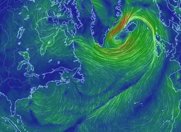
Rossby radius of deformation
• The Rossby radius of deformation (Ld) controls the typical length scale for ocean and atmosphere “weather”.
• Length scale at which rotational and stratification effects (i.e. vorticity advection and vortex stretching) are comparable.

 ℎ ′ 
 = =
 
 Atmosphere: Ld ~1000 km, period ~4 days Ocean: Ld ~10-200 km, period ~40 days
 Snapshot of surface winds Snapshot of surface currents

 October 29, 2014

 Image credit: earth.nullschool.net (forecast for 2020-03-16)

Assumptions:
 Geostrophic balance • Not on the equator (i.e. f >> 0).
 • Inertial terms are negligible (i.e. Ro > (1/f).

 Surface geostrophic currents follow sea-surface height contours.

 Combining geostrophic and hydrostatic balance* gives thermal wind balance:

• Horizontal gradients in density (easy to observe) determine vertical shear of
 currents (hard to observe).

• Geostrophic assumptions hold over much of the open ocean and many
 ocean observing systems rely on thermal wind (e.g. RAPID array at 26N). Image credit: Ocean Circulation 2nd Edition, The Open University

• Note that if density is a function of pressure only (i.e. barotropic), the
 geostrophic velocity is independent of depth. In this case geostrophic
 currents at all depths are determined by gradients in sea surface height.
 *note use of the Boussinesq approximation: i.e. density variations
 are ignored except where they appear in terms multiplied by g.
 EUROPEAN CENTRE FOR MEDIUM-RANGE WEATHER FORECASTS October 29, 2014

Assumptions:
 Ekman transports • As geostrophic, but with a frictional surface boundary.
 • Friction included as wind stress vector (τ), which represents
Inclusion of frictional terms results in a departure from vertical turbulent fluxes of horizontal momentum.
 • Frictional effects from wind stress contained within the
geostrophic balance near the ocean surface. Can split flow
 near-surface “Ekman layer” (i.e. τ(Zek) = 0).
into geostrophic and ageostrophic components:

 Thus depth-integrated Ekman flow is to the right (left) of imposed
 wind-stress in the northern (southern) hemisphere.

 (ageostrophic component)

Can avoid specifying the vertical distribution of stress by
integrating over the Ekman layer with appropriate
boundary conditions:

 Image credit: Ocean Circulation 2nd Edition, The Open University
 EUROPEAN CENTRE FOR MEDIUM-RANGE WEATHER FORECASTS October 29, 2014

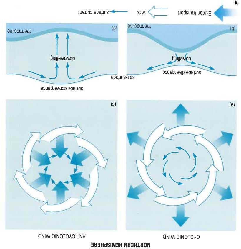
Assumptions:
 Ekman pumping • Within the Ekman layer, divergence of geostrophic current
 is small compared to divergence of Ekman transports.

Horizontal divergence of the integrated Ekman transports gives
rise to a vertical velocity at the base of the Ekman layer (i.e.
Ekman “pumping”):

Vertical velocities are a result of wind-stress curl (and
variations in f near the equator). In both hemispheres:

• Anticyclonic winds drive downwelling (Ekman pumping).
• Cyclonic winds drive upwelling (Ekman suction).

Divergence of Ekman transports also drives coastal and
equatorial upwelling/downwelling.

 EUROPEAN CENTRE FOR MEDIUM-RANGE WEATHER FORECASTS October 29, 2014
 Image credit: Ocean Circulation 2nd Edition, The Open University

Potential vorticity conservation
Potential vorticity (PV) is a quantity that is conserved with fluid flow
derived by combining conservation of mass and vorticity. For a layer
of constant density and thickness (H):

In the ocean interior, PV is conserved with fluid flow:
 Image credit: Atmospheric and Oceanic Fluid Dynamics 2nd Edition, Vallis

At the planetary scale, flow is constrained to follow f/H contours.
Stretching of a column (i.e. increased H) is balanced by increased
f (i.e. poleward motion).

PV conservation breaks down under the following conditions:
- Frictional boundaries
- Heating/cooling at the surface.
- Mixing across isopycnals (i.e. changing stratification).

 EUROPEAN CENTRE FOR MEDIUM-RANGE WEATHER FORECASTS Image credit: Ocean Circulation 2nd
 October 29,The
 Edition, 2014Open University

Assumptions:
 Sverdrup balance • Steady geostrophic flow in ocean interior (below Ekman
 layer, away from frictional boundaries).
Combine continuity equation with divergence of geostrophic • Forced from above by Ekman pumping/suction.
 • Assumed can integrate to a level of no motion where w=0
flow in the ocean interior:
 Now integrate from the base of the Ekman layer to the a
 known level of no motion (e.g. ocean floor):

 (Sverdrup relation)

This equation relates geostrophic currents to vertical Substitue wek and manipulate:
velocities and is an expression of (linearized) vorticity
balance.

Squashing (stretching) columns of water moves them
equatorward (poleward).

 We get an expression for the total depth-integrated meridional
 flow (Sverdrup transport) that is aOctober
 EUROPEAN CENTRE FOR MEDIUM-RANGE WEATHER FORECASTS function
 29, 2014of wind-stress only.

Wind-driven gyres However, Sverdrup theory does not predict the existence of a
 strong WBC - could also integrate from the western boundary.
 Can now define a streamfunction (Ψ) in terms of the zonal Western intensification of flow is a consequence of conservation
 integral of wind-stress curl that represents the 2D depth- of vorticity and requires the existence of ageostrophic terms (i.e.
 integrated flow: frictional boundary layers).

 Stommel (1948) and Munk (1950) developed models of the
 depth-integrated wind-driven flow that predict the existence of
 western boundary currents by including representations of
 linear drag and momentum diffusion, respectively.

 Integrating from the eastern boundary gives results consistent Munk gyres showing western boundary currents.
 with the existence of strong western boundary currents.

 EUROPEAN CENTRE FOR MEDIUM-RANGE WEATHER FORECASTS October 29, 2014
Image credit: Atmosphere, Ocean, and Climate Dynamics, Marshall & Plumb Image credit: Ocean Circulation 2nd Edition, The Open University

Wave fundamentals Wave basics

• Climatically relevant ocean waves propagate as perturbations to
the depth of the ocean thermocline.
• These phenomena can be modelled using the “reduced gravity”
shallow water equations.
• The density difference between layers is typically much less than
the reference density, so g’ ~ g / 300.
• 10 cm displacement of sea surface height associated with 30 m
displacement of the thermocline.
• Vertical density structure can (to some extent) be inferred from Image credit: Atmospheric and Oceanic Fluid Dynamics 2nd Edition, Vallis

satellite observations of sea surface height
 ~10 cm

 ( 2 − 1 ) ′ 
 = ′ = =
 1 

 ~30 m
 October 29, 2014

Assumptions:
 Quasi-geostrophic theory • Scale of flow similar to deformation length scale ( =
 
 ൗ ).
 • Close to geostrophic balance (Ro

Rossby waves
• Rossby waves are a consequence of latitudinal variations in planetary
 vorticity (i.e. f increases polewards).
 Rossby wave phase speed as a function of
• They are solutions to the linearized shallow water equations using the latitude in the ocean (Chelton et al. 1996)

 quasi-geostrophic approximation.

 • Phase velocity is always westwards relative to the zonal mean flow.

 • Group velocity (energy propagation) can be eastward or westward,
 depending on the zonal vs meridional scale of waves.

 • Waves travel faster closer to the equator and longer waves travel
 faster than shorter waves (dispersive).

 Rossby wave dispersion relation for reduced gravity model (no background flow)
 10 years to cross the Atlantic at 40N!

 October 29, 2014

Rossby waves: mechanism of propagation
• Propagation mechanism is a function of wavenumber relative to deformation radius (Ld).

• Short waves: balance between relative vorticity and planetary vorticity.

• Long waves: balance between vortex stretching and planetary vorticity

• Waves can be a mixture of both mechanisms.

 Propagation mechanism for short waves (i.e. f + ς = constant)

 October 29, 2014

 Image credit: Atmospheric and Oceanic Fluid Dynamics 2nd Edition, Vallis

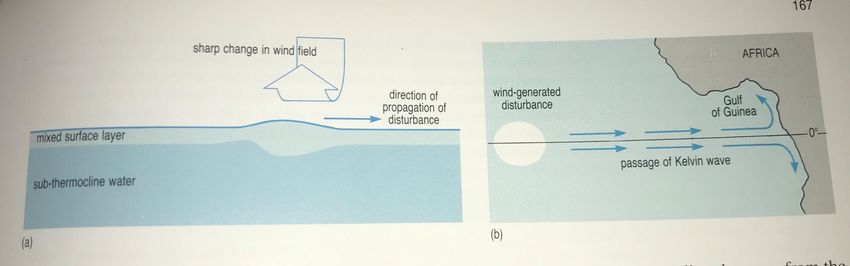
Kelvin waves
• Wave solutions to the linearized shallow water equations at a boundary.

• Waves are thus confined to coastlines and the equatorial waveguide.

• Propagate with a boundary to the right (left) in the northern (southern) hemisphere and travel eastward
along the equator.

• Kelvin waves are non-dispersive ( = = ′ )

• It takes about 2 months for the first baroclinic Kelvin wave to cross the equatorial Pacific (c ~ 3 m/s).

• Equatorial waves triggered by changes to the wind field are an important component of ENSO dynamics.

 October 29, 2014
 Image credit: Ocean Circulation 2nd Edition, The Open University

Instabilities Simulated Gulf Stream rings

• Flow in the ocean and atmosphere is not generally stable:
small perturbations give rise to growing unstable modes.

• Baroclinic instability:
 – Responsible for atmospheric weather systems and
 mesoscale ocean eddies.
 – Requires horizontal density gradients.
 – Available potential energy converted to kinetic energy.
 Image credit: NASA
 – Occurs preferentially at horizontal scales given by the
 Rossby radius of deformation (Ld).
 Tropical instability waves related to shear in equatorial currents

• Barotropic/shear instability:
 – Requires shear in background flow (e.g. jets).
 – Mean-flow kinetic energy converted to eddy kinetic
 energy.

 EUROPEAN CENTRE FOR MEDIUM-RANGE WEATHER FORECASTS October 29, 2014

 Image credit: Webb (2018), Ocean Science, vol 14.

Examples of air-sea interaction

EUROPEAN CENTRE FOR MEDIUM-RANGE WEATHER FORECASTS October 29, 2014

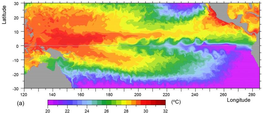
Air-sea interaction in the tropics
• Ocean-atmosphere variability in the tropics is strongly coupled.

• For example, changes in east-west sea-surface temperature (SST) gradients can impact deep convection and the
large-scale atmospheric zonal overturning circulation (Walker Cell).

• The resulting surface wind response impacts the ocean thermocline in way that amplifies the initial change to
east-west SST gradients, and thus reinforces the circulation response.

• This amplification is known as the Bjerknes feedback, and is an important part of the dynamics of the El Nino-
Southern Oscilation (ENSO) and Indian Ocean Dipole (IOD).

 EUROPEAN CENTRE FOR MEDIUM-RANGE WEATHER FORECASTS October 29, 2014
 Image credit: Wikipedia/NOAA/PMEL/TAO

Air-sea interaction in the mid-latitudes is scale-dependent
At scale basin of ocean basins, there is negative or zero correlation between SST and wind speed/heat fluxes
out of the ocean. Stronger winds → ocean heat loss → SST cooling → atmosphere driving ocean.

At scale of ocean fronts and eddies, there is positive correlation between SST and wind speed/heat fluxes out
of the ocean: Warmer SSTs → ocean heat loss → stronger winds → ocean driving atmosphere.

 Image credit: Chelton and Xie (2010)
 Image credit: Small et al. (2008)

A case where air flowing over an SST front experiences Relative orientation of prevailing winds and
enhanced mixing and downward transfer of momentum. SST gradients can impact wind stress curl and
 dirvergence.
 EUROPEAN CENTRE FOR MEDIUM-RANGE WEATHER FORECASTS October 29, 2014 33

Forecast challenges

EUROPEAN CENTRE FOR MEDIUM-RANGE WEATHER FORECASTS October 29, 2014

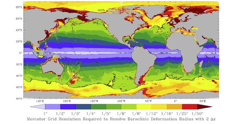
Forecast challenges: ocean model resolution
• It is necessary to resolve the Rossby radius of deformation (Ld) in order to accurately simulate sharp ocean fronts and mesoscale eddies.

• The operational configuration of the ECMWF ocean model has a resolution of 1/4th degree (~25 km): eddies are “permitted” in the lower
latitudes, but cannot be resolved in the mid-/high-latitudes or coastal regions.

• “Eddy resolving” configurations are very expensive (e.g. 1/12th degree costs 30 x more than 1/4th degree).

• This limits our ability to correctly simulate the position of the Gulf Stream and aspects of air-sea interaction.

 Image credit: Halberg (2013)

 EUROPEAN CENTRE FOR MEDIUM-RANGE WEATHER FORECASTS October 29, 2014

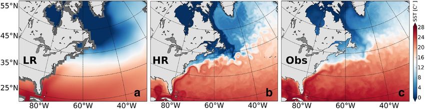
Forecast challenges: ocean model resolution
• Impact of ocean model resolution on the representation of the Gulf Stream

 100 km model resolution 10 km model resolution Observations

 Image credit: Siqueira and Kirtman (2016)

 EUROPEAN CENTRE FOR MEDIUM-RANGE WEATHER FORECASTS October 29, 2014

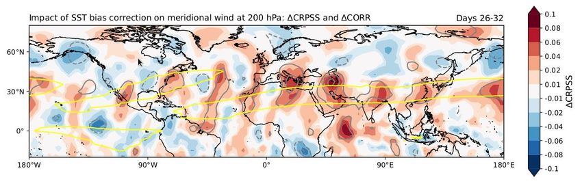
Forecast challenges: impact of Gulf Stream errors on ECMWF forecasts

 • The position of the Gulf stream influences the
 location, magnitude, and timing of upward
 motion and convection associated with cyclones
 propagating in the North Atlantic storm track
 (Minobe et al., 2008).
 • However, ocean models with a grid spacing of
 about 25 km, as used in the IFS, struggle to
 accurately simulate the location and structure of
 the Gulf Stream.
 • These errors can impact weather forecasts, with
 signals propagating out of the Atlantic along the
(a-b) Climatological SSTs seen by the atmosphere (contour spacing 2 K) and biases relative to ESA CCI
 northern hemisphere waveguide.
(c) Difference between BCFC and CTRL SST climatologies (shading). (d-e) Impact of North Atlantic SST
bias correction on the forecast skill of weekly mean anomalies in terms of CRPSS (shading) and anomaly • Higher‐resolution ocean models that can better
correlation (grey contour spacing of 0.1) for meridional wind at 200 hPa (v200). The yellow contours in
(e) highlight the position of the northern hemisphere waveguide diagnosed from the meridional gradient resolve the position of the Gulf Stream (grid
of absolute vorticity.
 spacing < 10 km) should improve future
Roberts et al. (2021), https://doi.org/10.1029/2020GL091446 ECMWF forecasts.

 EUROPEAN CENTRE FOR MEDIUM-RANGE WEATHER FORECASTS October 29, 2014 37

Forecast challenges: air-sea interaction
• Higher resolution ocean in coupled climate model simulates more intense air-sea interaction in regions of
high eddy activity, such as western boundary currents and the Antarctic Circumpolar Current.

• Simultaneous correlations between monthly mean SST and heat flux out of the ocean. Positive (red) values
are indicative of the ocean driving an atmospheric response.

 100 km model resolution 10 km model resolution

 Image credit: Kirtman et al. (2012)

 EUROPEAN CENTRE FOR MEDIUM-RANGE WEATHER FORECASTS October 29, 2014

Forecast challenges: ocean model initialization
• Accurate forecasts require accurate initial conditions.

• Full three-dimensional ocean state cannot be inferred from satellite data.

• Reliant on in situ observations from moorings, ship data, and profiling floats (e.g. Argo).

 • Since ~2004, the Argo network has measured
 temperature and salinity in the upper 2000 m with near
 global coverage.

 • It has revolutionized the ocean observing system, but it
 wasn’t designed to constrain the mesoscale (i.e. average
 spacing >> Ld)

 • Floats cycle to 2000m depth every 10 days.

 • Floats distributed over the global oceans (except on shelf
 seas and under ice) with an average spacing of ~300 km
 Image credit: argo.uscd.edu

 EUROPEAN CENTRE FOR MEDIUM-RANGE WEATHER FORECASTS October 29, 2014

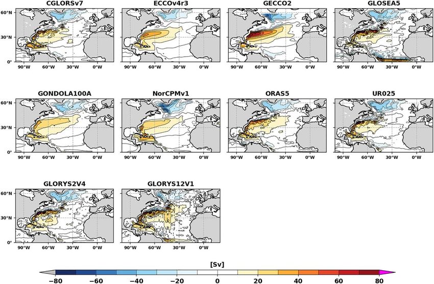
Forecast challenges: ocean model initialization
• Data assimilating ocean reanalyses are (arguably) less mature than their atmospheric counterparts, which is
reflected in the diversity of solutions in different products for key ocean properties.

• This is a consequence of (i) the small spatial scales that require very high resolution models, (ii) the
complexity of representing coastlines/bathymetry, and (iii) the difficulty of constraining the 3D ocean state from
observations.

 Barotropic stream functions in
 an ensemble of ocean
 reanalyses
 Image credit: Jackson et al. (2019)

 EUROPEAN CENTRE FOR MEDIUM-RANGE WEATHER FORECASTS October 29, 2014

Summary

EUROPEAN CENTRE FOR MEDIUM-RANGE WEATHER FORECASTS October 29, 2014

Summary
• Why is it important for ECMWF to model the ocean?
 – Processes: a dynamic ocean is necessary to represent key coupled ocean-atmosphere feedbacks.
 – Persistence: the large heat capacity of the ocean provides “memory” to the climate system.
 – Predictable dynamics: well-resolved and predictable ocean dynamics (e.g. equatorial waves) are important for ENSO
 and interannual variability.
 – Products: users are interested in the ocean state.

• Space and time scales of air-sea interaction:
 – Coupled ocean-atmosphere interaction occurs across huge range of spatial and temporal scales.
 – Processes that occur on timescales beyond our forecast horizon are still important as they must be correctly
 modelled in ocean/atmospheric reanalyses to provide accurate forecast initial conditions.

• Coupled forecasting challenges:
 – Accurate simulation of ocean boundary currents and mesoscale eddies requires significant increases in ocean
 resolution. This is computationally very expensive, which motivates the development of novel modelling approaches
 (e.g. reduced numerical precision, unstructured grids).
 – Model deficiencies and limitations of the ocean observing system result in biases and random errors in our estimates
 of the instantaneous ocean state used in forecast initial conditions. Reduction of these biases and improved
 representations of initial condition uncertainty (e.g. ocean stochastic physics) is important for accurate and reliable
 coupled forecasts.
 EUROPEAN CENTRE FOR MEDIUM-RANGE WEATHER FORECASTS October 29, 2014

References
Battisti, D. S., & Hirst, A. C. (1989). Interannual variability in a tropical atmosphereocean model: Mogensen, K., Keeley, S., & Towers, P. (2012). Coupling of the NEMO and IFS models in a single
Influence of the basic state, ocean geometry and nonlinearity. Journal of the atmospheric sciences, executable. Reading, United Kingdom: ECMWF.
46(12), 1687-1712.
 O’Neill, L. W., Haack, T., Chelton, D. B., & Skyllingstad, E. (2017). The Gulf Stream convergence zone
Chelton, D. B., & Schlax, M. G. (1996). Global observations of oceanic Rossby waves. Science, in the time-mean winds. Journal of the Atmospheric Sciences, 74(7), 2383-2412.
272(5259), 234-238.
 Parfitt, R., & Czaja, A. (2016). On the contribution of synoptic transients to the mean atmospheric
Chelton, D. B., & Xie, S. P. (2010). Coupled ocean-atmosphere interaction at oceanic mesoscales. state in the Gulf Stream region. Quarterly Journal of the Royal Meteorological Society, 142(696),
Oceanography, 23(4), 52-69. 1554-1561.

Colling, A. (2001). Ocean circulation 2nd Edition, The Open University. Butterworth-Heinemann. Rahmstorf, S. (2002). Ocean circulation and climate during the past 120,000 years. Nature,
 419(6903), 207-214
Hallberg, R. (2013). Using a resolution function to regulate parameterizations of oceanic mesoscale
eddy effects. Ocean Modelling, 72, 92-103. Roberts, C. D., Senan, R., Molteni, F., Boussetta, S., Mayer, M., & Keeley, S. P. (2018). Climate
 model configurations of the ECMWF Integrated Forecasting System (ECMWF-IFS cycle 43r1) for
Jackson, L. C., Dubois, C., Forget, G., Haines, K., Harrison, M., Iovino, D., ... & Piecuch, C. G. (2019). HighResMIP. Geoscientific model development, 11(9), 3681-3712.
The mean state and variability of the North Atlantic circulation: a perspective from ocean
reanalyses. Journal of Geophysical Research: Oceans. Siqueira, L., & Kirtman, B. P. (2016). Atlantic near‐term climate variability and the role of a resolved
 Gulf Stream. Geophysical Research Letters, 43(8), 3964-3972.
Johns, W. E., Baringer, M. O., Beal, L. M., Cunningham, S. A., Kanzow, T., Bryden, H. L., ... & Curry,
R. (2011). Continuous, array-based estimates of Atlantic Ocean heat transport at 26.5 N. Journal of Small, R. D., deSzoeke, S. P., Xie, S. P., O’neill, L., Seo, H., Song, Q., ... & Minobe, S. (2008). Airsea
Climate, 24(10), 2429-2449. interaction over ocean fronts and eddies. Dynamics of Atmospheres and Oceans, 45(3-4), 274-319.

Kirtman, B. P., Bitz, C., Bryan, F., Collins, W., Dennis, J., Hearn, N., ... & Stan, C. (2012). Impact of Suarez, M. J., & Schopf, P. S. (1988). A delayed action oscillator for ENSO. Journal of the
ocean model resolution on CCSM climate simulations. Climate dynamics, 39(6), 1303-1328. atmospheric Sciences, 45(21), 3283-3287.

Marshall, J., & Plumb, R. A. (2016). Atmosphere, ocean and climate dynamics: an introductory text. Trenberth, K. E., & Caron, J. M. (2001). Estimates of meridional atmosphere and ocean heat
Academic Press. transports. Journal of Climate, 14(16), 3433-3443.

Minobe, S., Kuwano-Yoshida, A., Komori, N., Xie, S. P., & Small, R. J. (2008). Influence of the Gulf Vallis, G. K. (2017). Atmospheric and oceanic fluid dynamics. Cambridge University Press.
Stream on the troposphere. Nature, 452(7184), 206-209.
 Webb, D. J. (2018). On the role of the North Equatorial Counter Current during a strong El Niño.
Mogensen, K. S., Magnusson, L., & Bidlot, J. R. (2017). Tropical cyclone sensitivity to ocean coupling Ocean Science, 14(4), 633.
in the ECMWF coupled model. Journal of Geophysical Research: Oceans, 122(5), 4392-4412.

 EUROPEAN CENTRE FOR MEDIUM-RANGE WEATHER FORECASTS October 29, 2014