An Open-Source Gaussian Beamlet Decomposition Tool for Modeling Astronomical Telescopes
←
→
Page content transcription
If your browser does not render page correctly, please read the page content below
An Open-Source Gaussian Beamlet Decomposition Tool for
                                                           Modeling Astronomical Telescopes
                                                                               Jaren N. Ashcrafta and Ewan S. Douglasb
                                                         a
                                                             Wyant College of Optical Sciences, University of Arizona, Tucson, AZ 85721
                                                                 b
                                                                   Steward Observatory, University of Arizona, Tucson, AZ 85721
arXiv:2106.09162v1 [astro-ph.IM] 16 Jun 2021

                                                                                                ABSTRACT
                                               In the pursuit of directly imaging exoplanets, the high-contrast imaging community has developed a multitude
                                               of tools to simulate the performance of coronagraphs on segmented-aperture telescopes. As the scale of the
                                               telescope increases and science cases move toward shorter wavelengths, the required physical optics propagation
                                               to optimize high-contrast imaging instruments becomes computationally prohibitive. Gaussian Beamlet Decom-
                                               position (GBD) is an alternative method of physical optics propagation that decomposes an arbitrary wavefront
                                               into paraxial rays. These rays can be propagated expeditiously using ABCD matrices, and converted into their
                                               corresponding Gaussian beamlets to accurately model physical optics phenomena without the need of diffraction
                                               integrals. The GBD technique has seen recent development and implementation in commercial software (e.g.
                                               FRED, CODE V, ASAP)1–3 but appears to lack an open-source platform. We present a new GBD tool devel-
                                               oped in Python to model physical optics phenomena, with the goal of alleviating the computational burden for
                                               modeling complex apertures, many-element systems, and introducing the capacity to model misalignment errors.
                                               This study demonstrates the synergy of the geometrical and physical regimes of optics utilized by the GBD
                                               technique, and is motivated by the need for advancing open-source physical optics propagators for segmented-
                                               aperture telescope coronagraph design and analysis. This work illustrates GBD with Poisson’s spot calculations
                                               and show significant runtime advantage of GBD over Fresnel propagators for many-element systems.
                                               Keywords: Gaussian Beamlet, High Contrast, Coronagraph Simulation

                                                                                          1. INTRODUCTION
                                               The purpose of a coronagraph is to block starlight, but allow the light from an exoplanet to pass to a detector.
                                               Many varieties of coronagraphs are employed on the ground and are planned in space, but the common denomi-
                                               nator between every variant is that they require exceptional optical models to accurately simulate approximately
                                               a part-in-one-billion sensitivity to Earthlike planets. Coronagraphs operate principally utilizing elements that
                                               interact with the wave nature of light. Consequently, current coronagraph design tools compute diffraction inte-
                                               grals of large arrays to accurately simulate the near-field (Fresnel Integral, Angular Spectrum) and the far-field
                                               (Fraunhofer Integral) performance.4–6
                                                   A possible improvement on current simulations, Gaussian Beamlet Decomposition (GBD) is an expeditious
                                               method of propagating a wavefront via a superposition of Gaussian beams as complex rays. This enables simul-
                                               taneous modeling of diffraction,7 tilt/decenter errors,8 and polarization.9 An arbitrary wavefront is decomposed
                                               into a finite set of Gaussian beamlets that, when coherently added, recreate the original wavefront. The generally
                                               astigmatic beamlet is fully parameterized by a central ray that tracks the position of a beamlet, and a complex
                                               curvature matrix that describes its waist radius and curvature. Both quantities can be propagated using geomet-
                                               rical raytracing(Fig 1), enabling fast diffraction calculations. GBD’s capacity to mimic the accuracy of Fresnel
                                               diffraction was recently presented by Harvey et al.1 In this work the authors demonstrated that GBD can model
                                               both far-field (point-spread functions, interferometers) and near-field (defocused point-spread functions, spot of
                                               arago) optical phenomena.
                                                  Further author information: (Send correspondence to J.N.A.)
                                                  A.A.A.: E-mail: jashcraft@email.arizona.edu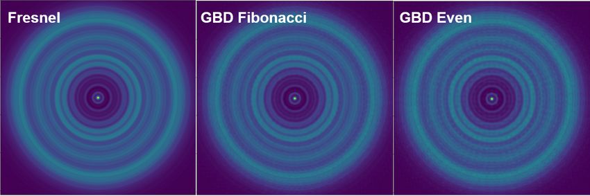
Gaussian beamlets are particularly useful in applications where absolute phase and diffraction effects are both
of interest. For example, in very high numerical aperture systems (e.g. microscopes) polarization effects limit the
accuracy of a typical scalar diffraction treatment.10 GBD can simultaneously model the scalar1, 11 and vector9
nature of optical fields, resulting in a more accurate physical optics model. GBD has largely seen implementation
in commercial optical design software (FRED, CODE V, ASAP) where it has been used as an analysis feature
in a variety of optical science investigations. In laser applications where gaussian beams are common, GBD
has been applied to study inter-cavity laser beam shaping.3 Astronomical telescope designers utilize GBD
to model interferometric instrumentation2, 12 and objectives with Gaussian foci in the far-infrared/milimeter
wavelengths.13 Recent efforts by Breckenridge and Harvey14, 15 utilized GBD in FRED to study the diffraction
features for different segmented-aperture geometries suited to optical telescopes outfitted with coronagraphs for
exoplanet detection.
   In this manuscript we describe the development of an open-source GBD module to provide telescope and
coronagraph designers with a new tool for modeling optical systems. The theory of GBD is introduced, and the
accuracy of the model in comparison to Fresnel Diffraction is presented, with further discussion on the potential
advantages of developing this platform of physical optics propagation in an open-source environment.

1.1 Parameters of the Gaussian Beam
The Gaussian Beam is a solution to the Helmholtz equation that takes the form16

                                                      Vo          r2
                                               V =        exp[ik       ]                                          (1)
                                                     q(z)        2q(z)

   Where Vo is the amplitude, k is the wavenumber, r is the radial coordinate in the plane perpendicular to
propagation, and q(z) is the complex valued constant that describes the beam’s 1/e field size (the ”waist” wo )
and curvature. This constant is referred to as the complex beam parameter.
                                                         1        λ
                                             q(z)−1 =        +i                                                   (2)
                                                        R(z)    πw(z)2

    q(z) is a convenient expression of the Gaussian beam because it fully encapsulates the information required
to describe the transverse electric field of the beam as it propagates. The real part of q(z) is related to the radius
of curvature (R(z)) of the wavefront.
                                                                Zo
                                                 R(z) = z(1 + ( )2 )                                               (3)
                                                                 z
Where Zo is the rayleigh range and z is the longitudinal propagation distance. The imaginary part is related to
the beam waist radius (w(z))                               r
                                                                   z
                                                w(z) = wo 1 + ( )2                                                 (4)
                                                                   Zo
For a generally astigmatic beamlet with different complex curvatures in orthogonal spatial dimensions, it is
convenient to define q(z) as a 2x2 matrix Q:
                                                         −1     −1

                                                  −1     q      qxy
                                                Q      = xx−1    −1                                               (5)
                                                         qyx    qyy

   The full expression of the generally astigmatic Gaussian beam is therefore:

                                                            −ik T −1
                                             V1 = Vo exp[      ~r Q ~r]                                           (6)
                                                             2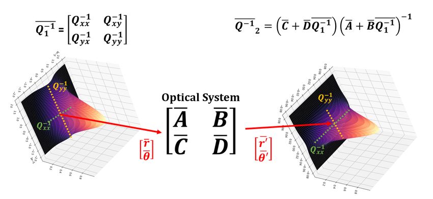
1.2 ABCD Ray Transfer Matrices
In the regime of geometrical optics, a generally skew ray can be traced through a system using 4x4 ABCD ray
transfer matrices.17 These matrices model simple optical elements (e.g. thin lenses) with ease by operating on
an input column vector that represents a light ray. The simplest ray transfer matrix that describes a paraxial
and orthogonal optical system is a 2x2 operator that maps an input (i) spatial and angular coordinate to the
appropriate output (o).
yo A B yi
= (7)
yo0 C D yi0
Where y is the spatial coordinate transverse to the propagation direction, and y 0 is the angle in that dimension.
In the orthogonal description, the elements of the ABCD matrix are real-valued scalars. To account for skew
ray paths, the position and angle in the dimension orthogonal to y and the direction of propagation must be
tracked, adding two dimensions to the matrix calculus. A nonorthogonal system with tilts and decenters that
map generally skew input rays to generally skew output rays is described by a 4x4 ABCD matrix.
xo Axx Axy Bxx Bxy xi
yo Ayx Ayy Byx Byy yi
0= (8)
Dxy x0i
xo Cxx Cxy Dxx
yo0 Cyx Cyy Dyx Dyy yi0
For simplicity, it is convenient to represent that radial position in the plane transverse to propagation (x,y)
and the corresponding angle in the dimension (x’,y’) as a position and angle vector respectively (~r, θ). ~ The
ABCD matrix can similarly be condensed into 2x2 sub matrices that operate on each spatial dimension, yielding
a familiar notation.
r~o A B r~i
= (9)
θ~o C D θ~i
This description is powerful because it communicates the elegance and simplicity of ray transfer matrices.
All dimensions transverse to propagation are accounted for, but the calculus to propagate a ray is still the
same. Similarly, the complex curvature of a generally astigmatic Gaussian beamlet can be propagated through
a nonorthogonal optical system using the 4x4 ABCD ray transfer matrix
−1 −1 −1 −1
Q2 = (C + DQ1 )(A + BQ1 ) (10)
This property of the complex beam parameter matrix is the cornerstone of Gaussian beamlet propagation.
The waist radius, beam curvature, and position can all be propagated using the linear laws of geometrical ray
tracing. This investigation will consider the propagation of Gaussian beamlets through thin lens elements (O) and
distances in a homogenous index of refraction (D), but other components (e.g. GRIN media, tilted/decentered
elements) have ABCD matrix equivalents that can be easily incorporated.8
1 0 0 0 1 0 dx /n 0
0 1 0 0 0 1 0 dy /n
O=
1/ef lx
;D = (11)
0 1 0 0 0 1 0
0 1/ef ly 0 1 0 0 0 1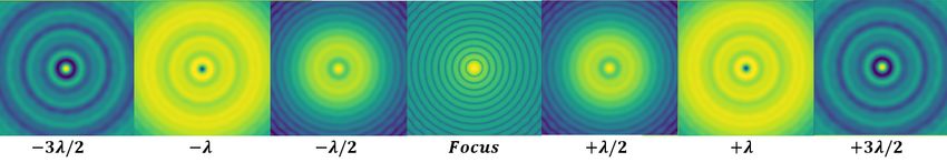
1.3 Complex Ray Tracing
A powerful property of the Gaussian beam is its ability to be propagated using the linear laws of geometrical
optics. Propagation of Gaussian beams via ray tracing was originally published by Arnaud in 1985 for laser
propagation.18 This technique enables complex field propagation through simple matrix multiplication, rather
than relying on computationally intensive Fourier transforms. The position of a Gaussian beam is tracked
                  ri θ~i )T that emanates perpendicular to the beam waist center and through the peak of the
by a central ray (~
beam. Propagating this ray through an ABCD Optical System matrix will return the position of the propagated
beamlet. The beam waist size and radius of curvature are then propagated through the same ABCD system via
                                   −1
the complex curvature matrix Q2 using equation 10 .

Figure 1. Gaussian beamlets are defined by a paraxial ”central ray” (shown in red) that locates the Gaussian beam, and
a complex curvature matrix that tracks the waist radius and curvature (Q−11 ). Utilizing the linear laws of paraxial ray
tracing, physical optics phenomena can be modeled.

   For a more general description of beamlet propagation from the input location r~i to the output location r~o ,
we look to the rigorous mathematics of Cai and Lin,19 who proposed the generally decentered and elliptical
Gaussian Beamlet (VDEGB ).

                                          −1                               ik T −1
                VDEGB = [det(A + BQ1           )]1/2 exp[−ikzo ] ∗ exp[−      r~o Q2 r~o ] ∗ exp[X] ∗ exp[Y ]      (12)
                                                                            2

   Where X and Y are the phase factors that arise from the beamlet decenter, reproduced below.

                                                     ik T      −1  −1
                                           X=−          r~i (Q2 + A B)~
                                                                      ri                                           (13)
                                                      2

                                                                  −1
                                                      ri T (AQ2
                                                Y = ik~                + B)r~o                                     (14)

    While the derivation of this expression was described by the authors as ”tedious but straightforward”, it
results in a powerful description of a key element in the GBD method: The ability to spatially decompose an
incident wavefront.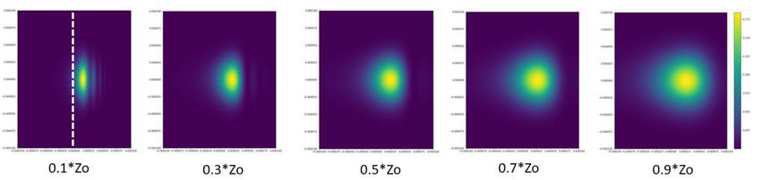
1.4 Gaussian Beamlet Decomposition
The decomposition of a wavefront into Gaussian beamlets requires a treatment of how the phase evolves with the
propagation of a decentered beamlet. This is because typical decomposition algorithms accomplish wavefront
decomposition through a distribution of beamlets in the entrance pupil of the optical system. Few methods have
been explored to best decompose an input wavefront into a finite set of Gaussian beams. The simplest method is
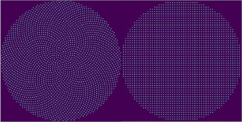
an even distribution of beams across the input wavefront (henceforth referred to as even sampling). The number
of Gaussian beamlets (Ngb ) across one dimension (W ) of the wavefront is given by
W ∗ OF
Ngb = . (15)
2wo
Where OF is the overlap factor of the beamlets. This factor describes the degree to which adjacent beamlets
overlap. Some partial overlap of adjacent beams is desirable to reduce the ripple that results from undersampling
the wavefront. However, an OF that is too high will result in a soft aperture edge, which low-pass filters the
input wavefront. Literature suggests that an OF = 1.5 − 1.71 is the appropriate range to experience the ripple
and low-pass filtering minimally. An alternative sampling method which yields a more efficient decomposition
for optical systems with rotational symmetry evenly distributes the beamlets on a Fibonacci spiral (henceforth
referred to as Fibonacci sampling).
Figure 2. Demonstration of various sampling schemes (Right) Even sampling1 (Left) Fibonacci sampling.11 (Top) Under-
sampling in pupil plane to show beamlet distribution, (Bottom) The corresponding PSF.
Both sampling schemes have been developed in the GBD code for comparison, given that each may be more
optimal for different system geometries. The Fibonacci sampling scheme is interesting because it has been shown
to result in lower RMS error to a flat wavefront for circular entrance pupils, which are very common for optical
systems.20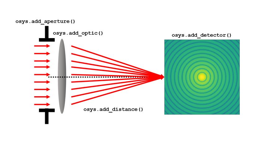
2. METHODS
In order to validate our approach, we baseline our systems in POPPY (Physical Optics Propagation in Python).
POPPY is an open-source project that simulates the behavior of complex scalar optical fields using numerical
FFT-based approaches.21 This project was originally developed as the physical optics engine for WebbPSF, a tool
developed to simulate the point spread functions of the James Webb Space Telescope (JWST) using Fraunhofer
diffraction. The capacity of this tool was later extended6 to incorporate Fresnel diffraction,22 which captures
both the near and far-field effects that limit high-contrast imaging systems.4 This implementation was used to
model the Magellan Extreme Adaptive Optics upgrade (MagAO-X23 ) but in order to model all the surfaces in
the system the run time is significant (' 1 min per run).
   An object-oriented approach to Gaussian beamlet decomposition was written in Python similarly to POPPY’s
Fresnel mode for demonstration. A Gaussian beamlet Wavefront class and an Optical System class were added,
with methods included to sufficiently generate an orthogonal optical system composed of paraxial lenses with
vignetting apertures.

             OpticalSystem Method                                         Description
                 add optic(efl)                            Adds a thin lens to ABCD system matrix
          add distance(distance,index)                         Adds a propagation distance d/n
            add aperture(shape,size)                            Add a ray-vignetting aperture
             add detector(size,npix)               Adds an analysis plane where diffraction calculation is done
                         Table 1. Description of current optical system methods for the GBD code.

     # I n i t i a l i z e t h e Gaussian b e a m l e t w a v e f r o n t and o p t i c a l system
     gwfr = GaubletWavefront ( wavelength =2.2 e −6, s i z e =2.4 , samplescheme= ’ f i b o n a c c i ’ )
     o s y s = G a u b l e t O p t i c a l S y s t e m ( epd =2.4 , dimd=5e −4, npix =512)

     # Add a c i r c u l a r o p t i c o f 5 . 5 2 meter f o c a l l e n g t h
     o s y s . a d d a p e r t u r e ( shape= ’ l y o t ’ , d i a m e t e r =2.4)
     osys . add optic ( e f l = 5.52)

     # P r o p a g a t e t o f o c u s and add a d e t e c t o r
     o s y s . a d d d i s t a n c e ( d i s t a n c e =5.52 , i n d e x =1)
     osys . add detector ()

Figure 3. (Top) Sample code to demonstrate the user-friendly & object oriented construction of the GBD module and
(Bottom) a graphical representation of what the code creates.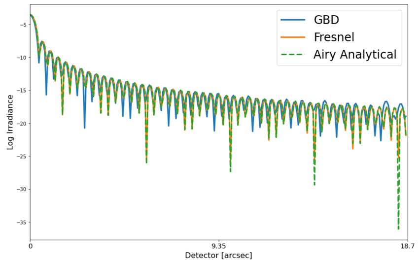
2.1 Accelerated Computing
Utilizing the iPython timeit function the propagator was profiled to identify the components that were critically
slowing runtime. The GBD code relies on computing the exponential of an array with dimensions [# pixels,#
pixels,# beamlets], as well as a for loop to construct the phase of each beamlet. For a large number of beamlets,
both numpy’s exponential and the phase construction loop become computationally prohibitive. To mitigate
the effects on runtime, two alternative acceleration methods were investigated. Numexpr24 is an accelerated
mathematical computing package for Python tailored to the processing of large arrays. Rather than handling
large arrays all at once numexpr computes the array in chunks to optimize computing time. Multi-threading
is also viable in numexpr for further enhancing performance. Numba25 is another accelerator for large array
computation that achieves performance enhancement by translating a numba decorated function into machine
code for increased computing performance. Numexpr produced the more expeditious exponential function (1.65x
Numba’s time), but is not able to process for loops. The phase construction loop was written as a function that
numba can accelerate, resulting in minimized computation time. By taking advantage of multi-threading compu-
tation can be accelerated further. For 90 threads the exponential of a complex array (dimension [512,512,2000])
was 1000x faster in numexpr than with numpy’s exponential on the same machine.

                                                     3. RESULTS
3.1 Far Field - The Airy Disk
One of the first problems introduced to students of physical optics is the solution to the Fraunhofer diffraction
integral for a circular aperture. This yields the familiar airy pattern, which is the basis for all images produced by
rotationally symmetric systems. Consequently, it is a powerful example for the comparison of different approaches
to diffraction calculations. The Fresnel and Fraunhofer diffraction integrals both have valid solutions to the focal
plane intensity. For sufficient validation of GBD’s far-field performance, we present a comparison of the airy
pattern generated by an ideal lens operating at a focal ratio of F/2.3 at a wavelength of λ = 2.2µm.

Figure 4. Cross-section of the focal plane intensity on a log scale generated by an ideal F/2.3 lens using Gaussian Beamlets
(blue) and Fresnel (orange) in comparison to the analytical airy function (green).

    The similarities in PSF structure between the three regimes of diffraction out to nearly the 50th airy ring are
compelling and indicative of GBD’s ability to preserve high spatial frequency content. This cements GBD as a
valid physical optics method for far-field diffraction calculations.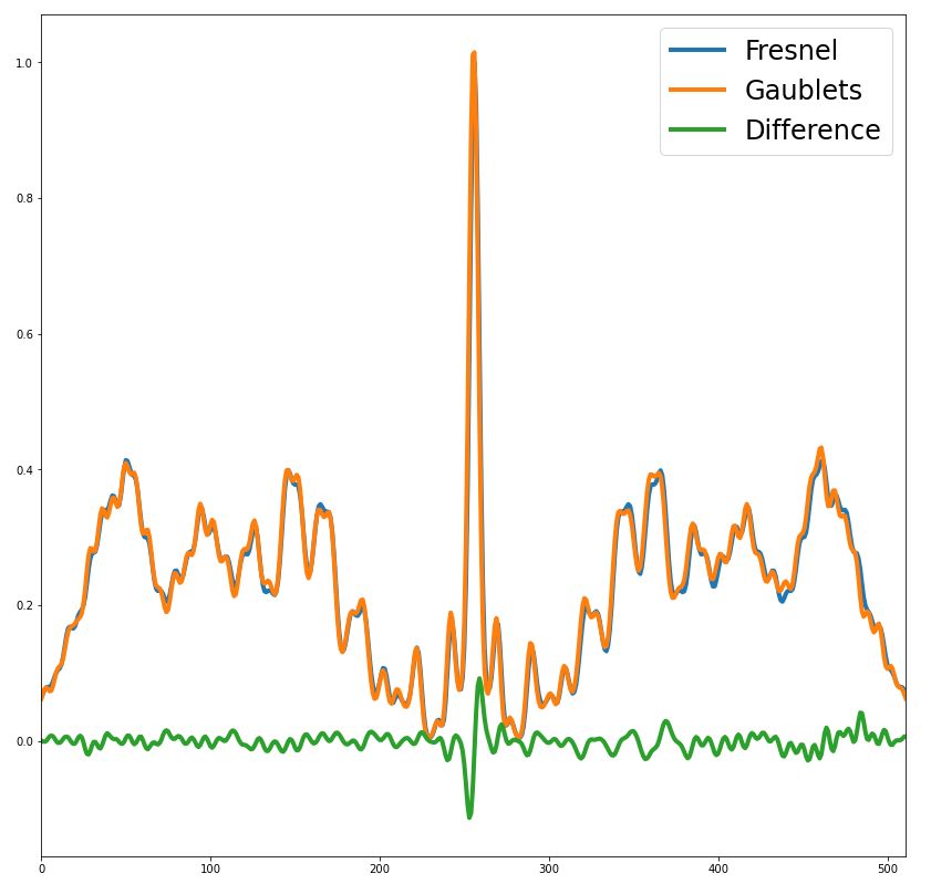
3.2 Near Field - Defocused PSF
The near-field regime of diffraction is much more challenging to model, but can capture many interesting physical
optics phenomena. One interesting feature is the behavior of the on-axis intensity of an airy disk as defocus
is added. Defocus (W020 ) is a field-independent aberration that scales quadratically with the pupil size. The
distance (L) corresponding to W020 waves of defocus is:

                                                     L = 8W020 λF 2                                                   (16)
Where F is the F-number of the optic. When light travels integer (n) waves of W020 from focus, the on-axis
irradiance goes to zero. Conversely, when light travels half-integer ((n + 1)/2) waves of W020 from focus, the
on-axis irradiance maximizes. This can typically only be modeled by direct propagation using Fresnel or Angular
Spectrum diffraction integrals. However, GBD is also capable of producing the same results.

Figure 5. Field intensity distribution near the focal plane at nλ/2 waves of defocus. The on-axis irradiance is expected to
maximize at half-integer waves of defocus and minimize at integer waves of defocus. Recovering this result using GBD is
proof that the method is capable of accurately modeling intensity distributions near the focal plane.

3.3 Near Field - Poisson’s Spot
Poisson’s spot is a phenomenon that can only arise with a physical optics treatment, making it another interest-
ing figure of comparison between existing physical optics propagators and GBD. When collimated light passes
through an annular aperture, a bright spot is seen on the axis that crosses through the innermost circular obscu-
ration. With a purely geometrical treatment this phenomenon is impossible because all light rays are parallel to
the optical axis. However, by virtue of diffraction the light near the aperture edges will constructively interfere
on-axis yielding the observed bright spot (Poisson’s Spot).26

Figure 6. Comparison of Poisson’s spot for cases of equal Fresnel number. (Left) POPPY’s Fresnel propagator. (Middle)
GBD propagator using Fibonacci sampling. (Right) GBD propagator using even sampling.
Figure 7. Cross-section of the Fresnel and GBD Fibonacci results from Fig 6 superimposed with the difference of the
Fresnel distribution with the GBD distribution.
Presented above are figures (Fig. 6,7) demonstrating the accuracy of GBD’s capacity to model near-field
propagation and Poisson’s spot relative to POPPY’s Fresnel propagator. Figure 6 provides a visual comparison
of the sampling schemes presented in section 1.4 to illustrate the ramifications of Gausian beamlet sampling.
The Fibonacci sampling scheme is clearly more suited to this problem than the even sampling scheme due to
the rotational symmetry of the aperture. The even sampling leaves much more apparent features of beamlet
distribution in the propagated field.
3.4 Runtime Comparison v.s. Poppy Fresnel Mode
To examine the current computational efficiency of GBD a comparison between the runtimes of POPPY’s Fresnel
mode and GBD at different beamlet samplings were examined. Due to the reliance on geometric propagation,
GBD’s runtime was fairly consistent for optical systems with 10-50 optical elements. Fresnel propagation relies
on a diffraction integral to propagate to each element, so the runtime scaled up as optical elements increased.
Figure 8. Comparison of runtime between GBD POPPY’s Fresnel mode for increasing number of optical elements. Due
to GBD’s reliance on raytracing for propagation, the runtime is dominated by the number of beamlets used rather than
the number of elements, making it ideal for many-element systems.4. FUTURE WORK
This work is intended to communicate the efficacy of a new physical optics propagator for open-source implemen-
tation geared toward the development of optical instrumentation for astronomical telescopes. We see potential
for substantive improvement of this code in the regimes of acceleration and more comprehensive modeling of
optical systems.
4.1 Tilt/Decentered ABCD Ray Transfer Matrices
Tilts and decenters of nonorthogonal optical elements can be accounted for by raising the rank of the ABCD
matrix to 5 and adding displacement terms in position (δx,δy) and angle (δx0 ,δy 0 ). To account for the increase
in rank a unit valued element is added to the ray vector.
xo Axx Axy Bxx Bxy δx xi
yo Ayx Ayy Byx Byy δy yi
0
δx0
0
xo = Cxx Cxy Dxx Dxy xi (17)
0 0 0
yo Cyx Cyy Dyx Dyy δy yi
1 0 0 0 0 1 1
This allows for the direct modeling of tilt and decenter errors in any component of a given ABCD system
matrix. Rudimentary results of a simple tilt and decenter of a thin lens have already been demonstrated by the
presented GBD code, but leveraging this feature of ray transfer matrices to do tolerance-informed optimization
of a physical optics model would be a powerful tool for diffraction-limited instrument design and development.
4.2 Truncated Gaussian Beamlet Decomposition
Accurate diffraction simulation of high spatial frequency physical optics phenomena (e.g. Fig 6) require a large
number of beamlets to produce a sufficient result. This is in part due to the low-pass filtering problem of GBD.
The beamlets at the edge of apertures do not fully capture the hard edge of an aperture, limiting the range of
spatial frequencies that can be captured by GBD. This is also observed in the PSF comparison (Fig. 4) where we
see a larger departure near the edge of the image (where the high spatial frequency content of the pupil is stored).
Sampling the aperture with smaller beamlets mitigates the roll-off at the edges, but results in a considerable
computational burdern (Fig. 8). Worku and Gross’s solution to this problem was to employ truncated Gaussian
beamlets in the decomposition phase. This expression of the Gaussian beamlet can be propagated geometrically
like the typical Gaussian beamlet, but captures more high spatial frequency information.
Figure 9. Propagation of a half-truncated Gaussian beam at fractions of the Rayleigh range. Observed here are the
near-field diffraction effects that result from capturing higher spatial frequency information at a hard aperture (white
dashed line).
4.3 GPU Acceleration
Greynolds27 recently published a manuscript indicating that there has been no implementation of GBD that
leverages the computational advantages of GPU-acceleration. The presented GBD code utilizes Numba25 to
assemble the phase of each beamlet one at a time. However, this calculation can be done in paralell on a GPU
by using NVIDIA’s CUDA,28 which is compatible with Numba. We anticipate substantive runtime decreases
that will enable higher sampling for a more comprehensive physical optics model of diffraction-limited systems.4.4 Alternative Sample Schemes
Current GBD methods utilize some uniform distribution (across an aperture or Fibonacci spiral) of beamlets
in the entrance pupil of the optical system. While simple to set up, this isn’t necessarily the most computa-
tionally efficient sampling scheme. Xia et al29 configured an optimization-based approach to compute a best-fit
generally astigmatic beamlet to the wavefront, subtract it, and repeat to generate a set of beamlets to prop-
agate that minimize the residual error. Greynolds30 discussed the expansion of GBD using a complete set of
Hermite-Gaussian or Laguerre-Gaussian polynomials to more completely reconstruct an arbitrary wavefront in
the entrance pupil. Both options are compelling for increasing the accuracy and decreasing the runtime of GBD,
and will be considered for addition with the development of the GBD module.
4.5 Polarization Ray Tracing for Vector Field Propagation
Previous investigations into GBD20 have illustrated the convenience of merging GBD’s scalar diffraction capa-
bilities with polarization ray tracing by assigning a Jones vector to the central ray to track the direction of
the electric field vector. The Jones vector is expressed in three dimensions: one in the direction of the central
ray, and the two directions transverse to the propagation vector (referred to as the s,p,k basis31 ). Different
electric field vectors can be assigned to every beamlet used in the decomposition. This enables users to as-
sign a spatially-varying polarization state across the input optical field, a feature not yet implemented in any
open-source field propagator. This is of particular interest to the high-contrast imaging community due to the
limitations polarization aberrations place on coronagraphs.15
4.6 POPPY Integration
This study was motivated by the desire to expand the capacity of POPPY by adding an alternative physical
optics propagation method to POPPY’s suite of Fraunhofer and Fresnel modes. With further optimization,
GBD’s performance and runtime may approach that of POPPY’s Fresnel mode. GBD also introduces the
capacity to model vector field propagation and misalignment errors; features which are not present in POPPY
currently. Successful formalization of the GBD code for integration into POPPY would result in a tool capable
of highly comprehensive physical optics modeling.
5. CONCLUSION
This manuscript presents the development of a new open-source platform for Gaussian beamlet decomposition
written in Python and verified against POPPY, an existing open-source physical optics code developed in the
context of astronomical telescopes. We demonstrate that GBD is capable of modeling both near and far-field
diffraction effects, and illustrate its potential for further development to model vector field propagation and
misalignment errors through polarization ray tracing and 5x5 ABCD matrices respectively. GBD’s synthesis
of geometrical propagation and high-fidelity diffraction simulation make it a worthy technique for the design
and analysis of future high-contrast imaging instruments,32 .33 A GitHub repository with the code used in this
investigation is published at Jashcraf/Gaussian-Beamlets.34
6. ACKNOWLEDGEMENTS
Portions of this work were supported by the Arizona Board of Regents Technology Research Initiative Fund
(TRIF). An allocation of computer time from the UA Research Computing High Performance Computing (HPC)
at the University of Arizona is gratefully acknowledged. The author also thanks Weslin Pullen for helpful
discussion throughout the duration of this study.REFERENCES
[1] Harvey, J. E., Irvin, R. G., and Pfisterer, R. N., “Modeling physical optics phenomena by complex ray
tracing,” Optical Engineering 54(3), 1 – 12 (2015).
[2] Stone, B. D. and Thompson, K. P., “Modeling interferometers with lens design software: beyond ray-based
approaches,” 74270A (Aug. 2009).
[3] Koshel, R. J., “Novel methods of intracavity beam shaping,” 47–57 (oct 2001).
[4] Krist, J. E., “PROPER: an optical propagation library for IDL,” in [Optical Modeling and Performance
Predictions III], Kahan, M. A., ed., 6675, 250 – 258, International Society for Optics and Photonics, SPIE
(2007).
[5] Soummer, R., Pueyo, L., Sivaramakrishnan, A., and Vanderbei, R. J., “Fast computation of lyot-style
coronagraph propagation,” Opt. Express 15, 15935–15951 (Nov 2007).
[6] Douglas, E. S. and Perrin, M. D., “Accelerated modeling of near and far-field diffraction for coronagraphic
optical systems,” in [Space Telescopes and Instrumentation 2018: Optical, Infrared, and Millimeter Wave],
Lystrup, M., MacEwen, H. A., Fazio, G. G., Batalha, N., Siegler, N., and Tong, E. C., eds., 10698, 864 –
877, International Society for Optics and Photonics, SPIE (2018).
[7] Harvey, J. E., Irvin, R. G., and Pfisterer, R. N., “Modeling physical optics phenomena by complex ray
tracing,” Optical Engineering 54(3), 035105–035105 (2015).
[8] Shaomin, W., “Matrix methods in treating decentred optical systems,” Optical and Quantum Electronics 17,
1–14 (Jan. 1985).
[9] Worku, N. G. and Gross, H., “Vectorial field propagation through high NA objectives using polarized
Gaussian beam decomposition,” in [Optical Trapping and Optical Micromanipulation XIV ], Dholakia, K.
and Spalding, G. C., eds., 33, SPIE, San Diego, United States (Aug. 2017).
[10] Mansuripur, M., “Distribution of light at and near the focus of high-numerical-aperture objectives,” Journal
of the Optical Society of America A 3, 2086 (Dec. 1986).
[11] Worku, N. G., Hambach, R., and Gross, H., “Decomposition of a field with smooth wavefront into a set of
gaussian beams with non-zero curvatures,” J. Opt. Soc. Am. A 35, 1091–1102 (Jul 2018).
[12] Dhabal, A., Rinehart, S. A., Rizzo, M., Mundy, L. G., Sampler, H. P., Juanola-Parramon, R., Veach, T. J.,
Fixsen, D. J., de Lorenzo, J. V. H., and Silverberg, R. F. F., “Optics alignment of a balloon-borne far-
infrared interferometer BETTII,” Journal of Astronomical Telescopes, Instruments, and Systems 3(2), 1 –
15 (2017).
[13] Narayananl, G., “Gaussian Beam Analysis of Relay Optics for the SEQUOIA Focal Plane Array,” 15th
International Symposium on Space Terahert Technology , 8 (2004).
[14] Breckinridge, J. B., Harvey, J. E., Hull, T., and Crabtree, K., “Exoplanet telescope diffracted light mini-
mized: the pinwheel-pupil solution,” in [Space Telescopes and Instrumentation 2018: Optical, Infrared, and
Millimeter Wave], MacEwen, H. A., Lystrup, M., Fazio, G. G., Batalha, N., Tong, E. C., and Siegler, N.,
eds., 61, SPIE, Austin, United States (July 2018).
[15] Breckinridge, J. B., Harvey, J. E., Irvin, R., Chipman, R., Kupinski, M., Davis, J., Kim, D.-W., Douglas,
E., Lillie, C. F., and Hull, T., “ExoPlanet Optics: conceptual design processes for stealth telescopes,” in
[UV/Optical/IR Space Telescopes and Instruments: Innovative Technologies and Concepts IX], Barto, A. A.,
Breckinridge, J. B., and Stahl, H. P., eds., 11115, 98 – 108, International Society for Optics and Photonics,
SPIE (2019).
[16] Goodman, J. W., “Introduction to fourier optics,” Introduction to Fourier optics, 3rd ed., by JW Goodman.
Englewood, CO: Roberts & Co. Publishers, 2005 1 (2005).
[17] Brouwer, W., “Matrix methods in optical instrument design.,” (1964).
[18] Arnaud, J., “Representation of gaussian beams by complex rays,” Appl. Opt. 24, 538–543 (Feb 1985).
[19] Cai, Y. and Lin, Q., “Decentered elliptical Gaussian beam,” Applied Optics Vol 41 No 21 , 5 (2002).
[20] Worku, N. G. and Gross, H., “Vectorial field propagation through high NA objectives using polarized
Gaussian beam decomposition,” in [Optical Trapping and Optical Micromanipulation XIV ], Dholakia, K.
and Spalding, G. C., eds., 33, SPIE, San Diego, United States (Aug. 2017).[21] Perrin, M. D., Soummer, R., Elliott, E. M., Lallo, M. D., and Sivaramakrishnan, A., “Simulating point
spread functions for the James Webb Space Telescope with WebbPSF,” in [Space Telescopes and Instru-
mentation 2012: Optical, Infrared, and Millimeter Wave ], Clampin, M. C., Fazio, G. G., MacEwen, H. A.,
and Jr., J. M. O., eds., 8442, 1193 – 1203, International Society for Optics and Photonics, SPIE (2012).
[22] Lawrence, G. N., “Optical Modeling,” in [Applied Optics and Optical Engineering. ], Shannon, R. R. and
Wyant., J. C., eds., XI, Academic Press, New York (1992).
[23] Lumbres, J., Males, J., Douglas, E., Close, L., Guyon, O., Cahoy, K., Carlton, A., Clark, J., Doelman,
D., Feinberg, L., Knight, J., Marlow, W., Miller, K., Morzinski, K., Por, E., Rodack, A., Schatz, L., Snik,
F., Gorkom, K. V., and Wilby, M., “Modeling coronagraphic extreme wavefront control systems for high
contrast imaging in ground and space telescope missions,” in [Adaptive Optics Systems VI ], 10703, 107034Z,
International Society for Optics and Photonics (July 2018).
[24] Cooke, D., Hochberg, T., Alted, F., Vilata, I., Wiebe, M., de Menten, G., Valentino, A., and McLeod, R. A.,
“NumExpr: Fast numerical expression evaluator for NumPy,” (Aug. 2018).
[25] Lam, S. K., Pitrou, A., and Seibert, S., “Numba: A llvm-based python jit compiler,” in [Proceedings of the
Second Workshop on the LLVM Compiler Infrastructure in HPC ], 1–6 (2015).
[26] Hecht, E., [Optics], Pearson (2012).
[27] Greynolds, A. W., “Ten years after (no, not the band): advancements in optical engineering computations
over the decade(s),” in [Novel Optical Systems, Methods, and Applications XXIII], Hahlweg, C. F. and
Mulley, J. R., eds., 10, SPIE, Online Only, United States (Aug. 2020).
[28] NVIDIA, Vingelmann, P., and Fitzek, F. H., “Cuda, release: 10.2.89,” (2020).
[29] Xia, D., “Fast Algorithm of Arbitrary Beam Propagation Based on Adaptive Elliptical Gaussian Beam
Decomposition,” IEEE , 2 (2019).
[30] Greynolds, A. W., “Fat rays revisited: a synthesis of physical and geometrical optics with Gaußlets,” in
[International Optical Design Conference 2014], Figueiro, M., Lerner, S., Muschaweck, J., and Rogers, J.,
eds., 9293, 521 – 529, International Society for Optics and Photonics, SPIE (2014).
[31] Yun, G., Crabtree, K., and Chipman, R. A., “Three-dimensional polarization ray-tracing calculus I: defini-
tion and diattenuation,” Applied Optics 50, 2855 (June 2011).
[32] Douglas, E. S., Ashcraft, J. N., Belikov, R., Debes, J., Kasdin, J., Lacy, B. I., Nemati, B., Milani, K.,
Pogorelyuk, L., Eldorado, A. J., Savransky, D., and Sirbu, D., “A review of simulation and performance
modeling tools for the Roman coronagraph instrument,” 11 (2020).
[33] Maier, E. R., Douglas, E. S., Kim, D. W., Su, K., Ashcraft, J. N., Breckinridge, B., Choi, H., Choquet, E.,
Connors, T. E., Durney, O., Guthery, C. E., Heath, J. C., Hyatt, J., Lumbres, J., Males, J. R., Matthews, E.,
Milani, K., N’Diaye, M., Noenickx, J., Ruane, G., Schneider, G., Smith, G. A., and Stark, C. C., “Design of
the vacuum high contrast imaging testbed for CDEEP, the Coronagraphic Debris and Exoplanet Exploring
Pioneer,” 17 (2020).
[34] Ashcraft, J. N., “Jashcraf/Gaussian-Beamlets: Working repository for GBD Manuscript SPIE AT+I 2020,”
(Dec. 2020).You can also read