Real Time Incremental Foveal Texture Mapping for Autonomous Vehicles
←
→
Page content transcription
If your browser does not render page correctly, please read the page content below
Real Time Incremental Foveal Texture Mapping for Autonomous
                                                                          Vehicles
                                                                              Ashish Kumar1 , James R. McBride2 , Gaurav Pandey2

                                                                                                                                  IMU                Sensors
                                         Abstract— We propose an end-to-end real time framework
                                         to generate high resolution graphics grade textured 3D map                        DGPS, Gyroscope,          Lasers,
                                                                                                                                                                   prior maps
                                         of urban environment. The generated detailed map finds its                         Wheel Encoders       Cameras, Radars
                                         application in the precise localization and navigation of au-
                                         tonomous vehicles. It can also serve as a virtual test bed for                                            Localization
                                         various vision and planning algorithms as well as a background
arXiv:2101.06393v1 [cs.CV] 16 Jan 2021

                                                                                                                           Obstacle Detection,
                                                                                                                                                  Path Planning
                                         map in the computer games. In this paper, we focus on two                            Classification
                                         important issues: (i) incrementally generating a map with
                                                                                                                                                     Control
                                         coherent 3D surface, in real time and (ii) preserving the
                                         quality of color texture. To handle the above issues, firstly,
                                         we perform a pose-refinement procedure which leverages
                                         camera image information, Delaunay triangulation and existing
                                         scan matching techniques to produce high resolution 3D map
                                         from the sparse input LIDAR scan. This 3D map is then                               Fig. 1: Autonomous Navigation System
                                         texturized and accumulated by using a novel technique of
                                         ray-filtering which handles occlusion and inconsistencies
                                         in pose-refinement. Further, inspired by human fovea, we
                                         introduce foveal-processing which significantly reduces                   Hence, it becomes crucial to acquire high quality textured
                                         the computation time and also assists ray-filtering to                    3D maps of the environment for a safe and robust operation
                                         maintain consistency in color texture and coherency in 3D                 of autonomous vehicles.
                                         surface of the output map. Moreover, we also introduce tex-                  Typically, the textured maps are generated by manually
                                         ture error (TE) and mean texture mapping error (MTME),                    driving a surveying vehicle endowed with LIDARs, GPS/INS
                                         which provides quantitative measure of texturing and overall
                                         quality of the textured maps.                                             and cameras through the environment/area to be mapped. In
                                                                                                                   general, the LIDAR is a short range device which provides
                                                                 I. I NTRODUCTION                                  a sparse 3D measurements. Hence, in order to generate a
                                            Recent advances in the sensor technology ([1], [2]) and                dense map of the environment, two approaches exists: (i)
                                         a breakthrough in real world algorithmic visual inference                 acquire the scans of the area from different physical locations
                                         ([3], [4], [5], [6], [7]) has brought the fully autonomous                and accumulate them into a local frame by a standard
                                         navigation/driving one step closer to the reality, perhaps most           simultaneous localization and mapping (SLAM) algorithm
                                         visible in ([8], [9], [10]). In this work, we focus on urban              ([16], [17], [18], [19], [20]) or (ii) exploit the camera images
                                         maps for localization of an autonomous navigation system                  for dense reconstruction of the map using bundle adjustment
                                         (ANS).                                                                    [21], [22], [23].
                                            Autonomous navigation system is fairly complex and                        Generating a detailed texture map of the environment is a
                                         consists of several modules as shown in fig. 1. In an ANS,                challenging problem mainly due to sparsity in LIDAR scans
                                         localization ([11], [12], [13]) happens to be one of the critical         and inconsistency in pose estimation due to complex trajec-
                                         tasks, as it provides vehicle’s location in the navigating en-            tories which sometimes are hard to optimize using SLAM.
                                         vironment. Although, centimeter accurate Global Positioning               Moreover, occlusion of 3D points in between LIDAR and
                                         System (GPS) and Inertial Navigation System (INS) ([14],                  camera frame appears as a bottleneck for detailed texture
                                         [15]) are available but they are often quite expensive. More-             mapping. It arises due to different physical mounting loca-
                                         over, these costly and high accuracy GPS technologies fail in             tions of LIDAR and camera. Hence, in this paper, we propose
                                         urban environment (due to multi-path error) and in regions                an end-to-end real time framework which performs multi
                                         where the line-of-sight to the GPS satellites is blocked (e.g.            modal sensor data fusion (LIDAR scans, images, navigation
                                         tunnels, underpasses, tree canopies etc.), resulting into a               data) to generate highly accurate, detailed textured 3D maps
                                         GPS-denied environment. In these scenarios, a vehicle/robot               of urban areas while simultaneously handling the problems
                                         registers the current sensor data (LIDAR/camera) with the                 of occlusion and pose inconsistency. The framework outper-
                                         map of the environment (prior maps) to localize itself.                   forms recent work [21], [24] and achieves map error below
                                                                                                                   5cm (in some cases 1cm).
                                            1 Mr. Ashish kumar is with the Department of Electrical Engineering,
                                                                                                                      The proposed framework (Fig. 2) consists of a novel
                                         Indian Institute of Technology, Kanpur krashish@iitk.ac.in                pose-refinement (Sec. III-A) technique which facil-
                                            2 Dr. James R. McBride and Dr. Gaurav Pandey are with Re-
                                         search & Innovation Center, Ford Motor Company [jmcbride,                 itates high fidelity pairwise scan matching and produces
                                         gpandey2]@ford.com                                                        accurately aligned dense version of input sparse scans. Once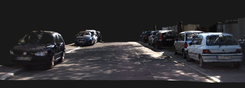
perform in real time due to its exhaustive computationally
                                                                           intensive steps (Table I). Whereas, the proposed upsampling
                                                                           technique performs in real time while approximately pre-
                                                                           serves the underlying surface.
 (a) Before pose-refinement           (b) After pose-refinement               LIDAR data becomes unreliable as target distance in-
                                                                           creases and appears as major source of noise in the mapping
                                                                           process. To cop with this, we refer to the working of foveal
                                                                           vision in the human visual cortex. In this domain, the success
                                                                           of the attention based deep learning architectures for object
       (c) Foveal extraction                  (d) Upsampling               detection [29], [30], [31], encourages us to employ foveal
                                                                           vision but we use it in an entirely different manner.
                                                                              The work in [32] and [33], [34], [35] proposes batch
                                                                           and incremental approaches respectively for texture map-
                                                                           ping. The former performs the mapping by accounting all
  (e) Foveal textured point cloud   (f) Corresponding ground truth image
                                                                           the viewing rays where as, the latter reconstruct the map
        Fig. 2: Major components of the framework                          incrementally by estimating boundary between free space
                                                                           and matter i.e. space carving. [21] uses tracking of image
                                                                           edge points to incrementally reconstruct a less detailed map
the dense 3D point cloud is obtained, we use a novel                       of the environment. Similar to us, [24] jointly estimate a 3D
ray-filtering (Sec. III-C) technique to transfer color                     map of the environment by using LIDAR scans and images.
texture into the aligned scan and accumulate it in such a                  However, they follow batch reconstruction in contrast to the
way that output map shows a high degree of coherent surface.               proposed work which is incremental in nature. Moreover,
This step only processes the foveal regions (2D and                        both [21] and [24] output a 3D mesh while the method
3D) defined by the novel foveal-processing concept                         proposed in this paper estimates a dense point cloud. [24]
which we have introduced in the sec. III-B and is inspired                 discards moving objects such as pedestrian or bicycles. It
from human fovea. This concept enhances the overall speed                  also proposes a novel way to incrementally estimate the
of the framework and improves the quality of the output map.               texture which is only evaluated qualitatively because in the
Further, we introduce two new metrics to asses texture and                 previous literature, a quantitative metric to asses texture
overall quality of the map which are discussed in the sec.                 quality doesn’t exist. In this work we propose such a metric
III-D. In the next section, we give an overview of the various             and focus mainly on improving the overall map quality while
topics involved in the design of this framework.                           leaving the moving object handling for future extension of
                                                                           the work.
                       II. R ELATED W ORK
   A prevalent approach for the pose estimation is to use                                     III. M ETHODOLOGY
SLAM ([16], [17], [18], [19], [20]), which requires all
                                                                           A. Pose Refinement
the data apriory. However, pose estimation can also be
done by using scan matching techniques such as Standard-                      Typically, a LIDAR can provide 3D world measurements
ICP [25], Point-to-Plane-ICP [26], Generalized-ICP [27].                   in a radii of ∼ 100m and these measurements are made w.r.t
The Standard-ICP minimizes point to point error (euclidean                 a vehicle/body frame (V ). Hence for larger maps, the LIDAR
distances) while Point-to-Plane-ICP minimizes distance be-                 scans need to be accumulated w.r.t. a fixed/local reference
tween a point and a locally estimated plane. GICP combines                 frame (L). However, the relative position of V w.r.t. L i.e.
point-to-point and point-to-plane metric and achieves state-               pose , is governed by the GPS/INS data which itself is noisy
of-the-art results. In this paper, we choose to estimate the               and unreliable. Hence, scan accumulation by using the raw
poses using scan matching techniques while focus remains                   poses leads to very unpleasant 3D structures (car, building,
on improving their accuracy. We do this due to two facts: (i)              wall) in the output map (Fig. 3g).
scan matching performs better for better initial guess as well                We handle this by performing pose-refinement
as for the lesser distances between scans to be aligned and (ii)           where we aim to register pair of LIDAR scans so that the
the state-of-the-art sensors (e.g. LIDAR, camera, INS/GPS)                 registered clouds can exhibit high degree of coherent surface
can provide data typically at the speed of ∼ 10fps. Due                    [36]. In order to achieve this, first we perform constrained
to the real time acquisition, LIDAR scans are separated by                 upsampling of each scan i.e. upsample only the non-ground
relatively short distances (∼ 0.5m) and INS/GPS data can                   points. We perform this minor yet useful tweak due to the
serve as a better initial guess for scan alignment.                        fact that the ground plane covers major area in a LIDAR scan
   The existing scan matching algorithms are point hungry                  and an upsampled ground plane may leave the registration
and upsampling often leads to improved scan matching                       algorithm trapped in local minima. In our case, we extract the
performance. [28] uses local plane to estimate underly-                    ground plane by using z thresholding as it is fast and works
ing surface using moving least squares and upsample the                    well at least locally. However, other approaches such as plane
surrounding of the point uniformly. However, it does not                   extraction using RANSAC [37] can also be exploited.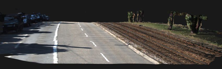
Restricted FOV                      Actual FOV

                                                                                                                 far blind zone
                                                                                                                   white zone
                                                                                                                     r blind zone
     (a)              (b)          (c)     (d)      (e)        (f)                                                nea

                 (g)                                  (h)                     (a) Top view                    (b) Side view

Fig. 3: (a) raw scan-pair (red-blue), (b) aligned scans using        Fig. 4: This figure shows the restricted field of view (FOV)
baseline GICP, (c)-(f) pose-refinement for upsampling                of cameras, white zone, near and far blind zones used for
rates 0, 1, 2, and 3 respectively. Figure (g) an accumulated         texture mapping.
point cloud of an area by using raw poses (odometry) and
(h) refined poses using pose-refinement.
                                                                     B. Foveal Processing
                                                                        Through experimental observation, we have noticed that
   Although, upsampling a point cloud is non-trivial, we             the farther points does not receive a fine grained color
devise a fast and intuitive way to achieve this. First, we obtain    texture due to sparsity, noise in LIDAR scans and large
image projection (pixel location) of LIDAR points using pin          angle (≥∼ 70o ) between view point and normal at the point.
hole camera model and triangulate all the image projections          Moreover, due to external factors e.g. sunlight, reflective
using Delaunay triangulation. Later, for each triangle t in          surface, the color texture of the objects in the images changes
pixel space, we retrieve a triangle T in 3D space. Now, we           drastically as the vehicle navigate through the environment
insert a new vertex which is the image projection of the             (Fig. 5). In such cases, approaches such as [24] doesn’t
centroid of the triangle T . It is noteworthy that this operation    preserve texture due to weighted averaging (kindly refer to
essentially upsamples the point cloud due to insertion of new        [24] for further details) in their texturing process. Hence,
vertices into the Delaunay triangles and number of repetition        inspired from human fovea [38], where major processing
of this step is equal to upsampling rate. We perform the             happens in a relatively smaller region of visual field, we
insertion operation only for the triangles T whose edges are         define similar regions by restricting field of view (FOV) of
below a threshold τ = 0.3m as otherwise it may give rise to          the camera to a thin horizontal and a thin vertical slice (2D
unwanted edges which physically are not present. The above           foveal region). Moreover, we also define a spherical
discussed upsampling technique obtains a smooth surface in           near blind, white and far blind zone (3D foveal region)
negligible time as compared to upsampling using [28] (Table          around the car (Fig. 4). The texture mapping is performed
I). The smoothness in the point cloud is evident from the fact       only in the white zone whereas it is avoided in the blind
that we use averaging operation while inserting a new vertex         zones because the near blind zone encloses vehicle itself
into the Delaunay triangles.                                         and the far blind zone have noisy depth measurements.
                                                                     The restricted FOV, various blind and white zones together
                                                                     improves the quality of texture mapping drastically and
                                   TABLE I:                          simultaneously improves algorithmic speed due to reduced
   Timing performance (CPU) of upsampling using proposed and [28]
                                                                     number of points, which are to be processed.
    order of points          10k     30k    90k     180k     450k
         [28]                 2s     15s    160s   1450s    10000s      Further, as soon as an aligned scan becomes available,
       proposed             30ms    60ms   120ms   300ms    900ms    its foveal region is extracted (Fig. 2e) which is upsam-
                                                                     pled including the ground plane and is operated by the
                                                                     ray-filtering discussed below.
   Further, the upsampled scans are aligned (registered) using
GICP [27] with the raw poses as initial guess. From fig. 3,          C. Ray-filtering and Texture Mapping
it can be seen that the constrained upsampling leads to a               The ray-filtering operation plays an important role
coherent registered surface which is rich in contextual 3D           in obtaining a fine grained texture in the map. This operation
information such as 3D edges, corners, walls etc. We also            discards the points PS in the scan S which if added to the
verify this experimentally in sec. IV.                               accumulated cloud (from previous scans), gets occluded or
   As we have discussed that the pose-refinement                     occludes any existing point in the accumulated cloud. In
also uses GICP as underlying scan matching technique,                general, such situations arise due to inconsistencies in the
we differentiate between pose estimation using standalone            pose and must be handled so as to maintain coherent 3D
GICP and pose-refinement by referring the former as                  surface in the output map.
a “baseline”. We maintain this keyword throughout the paper.            To achieve this, first we extract all the points PAf that lie
                                                                     in the foveal region of current pose. Next, a virtual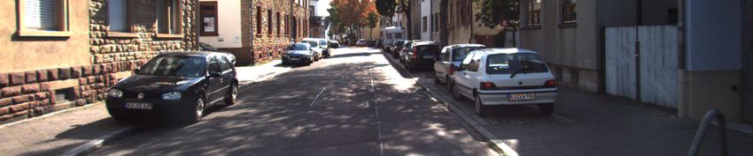
I                                  I

                                                                                          y      W                           y      W

                                                                                      C          z                       C         z
       (a) Frame 210           (b) Frame 220           (c) Frame 228
                                                                                  x                                  x
Fig. 5: Notice how the sunlight affects color texture of the
car as the surveying vehicle navigates from figure (a) to (c).
Frames taken from KITTI sequence 0095.                                                (a) Case of occluded                 (b) Case of occluding

                                                                                 Fig. 6: The figure above describes different ways, the
                                                                                          points can be occluded or occluding
ray from each point P in {PS , PAf } is emanated towards
camera origin (Fig. 6) and all of the such rays are projected
into the camera using the pin-hole camera model1 . However,
collinearity of rays or high density around a point sometimes
result in a common pixel projection (p) for multiple rays. To
handle this case, we assign p to a ray having shortest ray-                        (a) Frame 0               (b) Frame 0                (c) Frame 0
length d among all such rays. If d corresponds to a PS , it is
discarded as this happens to be the case of occluding.
   Further, to test the case of occluded, we take a window
(W) of size [M × M ] centered at the image projection p of
                                                                                  (d) Frame 20               (e) Frame 20               (f) Frame 20
each PS (Fig. 6). Now, we compute mean (µ) and standard
deviation (σ) (Eq. 1) of all the ray-lengths di s inside the
window and perform a statistical outlier rejection test (Eq.
2) on them in order to obtain an outlier score. If the outlier
score is less than an outlier rate c, the point Pt is marked
as visible otherwise it is considered as occluded. In general,
lesser the value of c, higher will be the rejection rate i.e.
                                                                                      (g) Frame 20 − 40                      (h) Frame 20 − 40
more number of points will be marked as occluded. Hence,
frequency of inliers in a window can be controlled by varying                 Fig. 7: Zoom in for better insight. Figure (a), (d) ground
the value of c.                                                               truth patch images. Corresponding patches of textured point
                                  N                                           cloud using (b), (e) baseline texturing and (c), (f) proposed
                               1 X                                            texturing. (g) textured point cloud using baseline, and (h) us-
                        µ=           di
                               N i=1                                          ing proposed texturing. Frames taken from KITTI sequence
                              N
                                                                       (1)    0095.
                         2 1 X             2
                       σ =       kdi − µ)k
                           N i=1
                         (                                                    the points and classify the 3D space as matter or void by
                             V isible,      if |diσ−µ| ≤ c                    ray-intersection.
               PS is =                                                 (2)
                             Occluded,      Otherwise                         D. Error Metrics
Where, N 6 M × M is total number of rays projected in                            Authors in the previous works [21], [24] have reported
the window.                                                                   the quantitative map error (M E, Eq. 3), which is mean
   Now, we texturize the filtered points from S by pro-                       (µM E ) and standard deviation (σM E ) of euclidean distances
jecting them into the image and later add them to the                         between the points and their ground truth. This metric
accumulated cloud. Unlike [24], [39] in which color tex-                      provides a measure for the quality of the 3D surface of the
turing is a weighted averaging operation (low pass filtering)                 map but it does not convey anything about the quality of
and doesn’t preserve sharp edges, the visibility test using                   texture. Therefore, in this work we propose a quantitative
ray-filtering inherently preserves the image texture                          error metric for texture quality of the map. We propose
information resulting in fine grained texture detail in the                   two error metrics (i) texture error (T E, Eq. 4) and (ii)
textured map (Fig. 7).                                                        mean texture mapping error (M T M E, Eq. 5). The
   If a PS passes both the tests, it represents the case of space             former is the mean (µM E ) and standard deviation (σM E )
carving. The ray-filtering performs it in an entirely                         of euclidean distances between the intensity/RGB of points
different manner as no triangulation or any ray-intersection                  and their ground truth. While the latter is an averaged sum
test is performed in contrast to [33], [35], which triangulate                of product of euclidean distances between 3D location and
                                                                              intensity/color of the points and their ground truth. For
  1p   = K[R|t]P , where K, R | t are intrinsic and extrinsic camera matrix   texture mapping purpose, T E, M T M E are computed over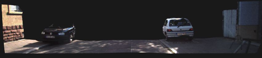
all the points in the original LIDAR scans. Both T E and
M T M E provides quantifiable measures to assess the texture
and overall quality of textured maps. We have experimentally
demonstrated the usefulness of both T E and M T M E in the
section IV below.                                                       (a)           (b)                 (c)             (d)

                        n   ki
                     1 X X
           µM E    =              PjL − PnM
                     N i=1 j=1
                        n   ki
                                                         (3)
            2        1 X X                       2                      (e)           (f)                 (g)             (h)
           σM E    =              PjL   − µM E
                     N i=1 j=1
                                                               Fig. 8: (a),(c),(e),(g) scan aligned using baseline GICP, and
                                                               (b),(d),(f),(h) pose-refinement with GICP + 3xUp
                        n   ki
                     1 X X
           µT E =                 CjL − CnM
                     N i=1 j=1
                        n   ki
                                                         (4)
                     1 X X                       2             rates 0xUp2 , 1xUp, 2xUp, 3xUp. We also report timing
           σT2 E   =              CjL − µT E                   performance (CPU) averaged over the number of frames in
                     N i=1 j=1
                                                               the respective sequence. We compare our results with those
                 n   ki                                        achieved by the standalone baseline GEN-ICP, STD-ICP, and
              1 X X
 MTME =                     PjL − PnM . CjL − CnM        (5)   P2P-ICP, the navigation data serves as initial guess for all
              N i=1 j=1                                        the experiments
where                                                             In the sequence 0095, the STD-ICP, P2P-ICP fails to
  ki   total number of points in ith LIDAR scan                converge and show higher average error3 (Fig. 10a), however,
  PjL
       j th point in LIDAR scan                                with pose-refinement both of them converges for the
    M                                                          complete sequence which indicates the effect of the proposed
  Pn   nearest neighbor of PjL in the map
    L                                                          method. For the sequence 0001, the baselines and 0xUp
  Cj   intensity I or color [R, G, B] of PjL
    M                                                          have similar registration error which decreases as upsam-
  Cn   intensity I or color [R, G, B] of PnM
                                                               pling factor is increased (Fig. 10a). Averaged over all the
  µM E mean of the map error
                                                               scan matching techniques, the point-to-point error (m) for
  σM E standard deviation of the map error
                                                               seq 0095, decreases from 0.14 (baseline) to 0.08 (0xUp),
  µT E mean of the texture error
                                                               0.06 (1xUp), 0.03 (2xUp) 0.023 (3xUp) and for seq 0001,
  σT E standard deviation of the texture error
                                                               it decreases from 0.12 (baseline) to 0.118 (0xUp), 0.115
  n   PTotal  number of scans
         n                                                     (1xUp), 0.10 (2xUp), 0.08 (3xUp). Though, the difference
  N = i=1 ki
                                                               between maximum and minimum registration errors is ∼
            IV. E XPERIMENTS AND R ESULTS                      0.12m (seq 0095) and ∼ 0.03m (seq 0001), the small
                                                               improvement has large positive effects on the 3D surface
   We validate the performance of the proposed framework       quality of the generated maps (Fig. 8). Hence, we argue that
against the publicly available KITTI dataset [40]. Our focus   the upsampling leads to a better scan-matching performance
in this paper has remained on generating high resolution       and it also improves the quality of the texture map. Further,
textured maps. Hence, from the dataset we only choose          fig 10b, 10b shows the scan matching timing performance
the sequences having minimal number of moving objects,         of the baselines and the pose-refinement for various
in particular, sequence 0095 (268 frames) and 0001 (108        upsampling rates. We average the time over the number
frames). Each sequence has time synchronized frames, each      of frames in the respective sequence and observe that the
of which contains LIDAR scans captured by velodyne HDL-        time consumed for alignment is directly proportional to the
64E, RGB image of size 1242x375 captured by Point Grey         number of points. Further, the keyword “real-time” in this
Flea 2 and navigation data measurements by OXTS RT             paper refers that all modules of the algorithm except the scan
3003 IMU/GPS. All the experiments were performed on a          alignment process execute in real time on the given CPU.
computing platform having 2 x Intel Xeon-2693 E5 CPUs,         However, a GPU version of the scan alignment algorithms
256 GB RAM, 8 x NVIDIA Geforce GTX 1080Ti GPUs.                can be used to achieve overall real time performance. Since
A. Scan Matching Performance and Timing Analysis               our intention in this paper has been to improve the mapping
                                                               and texture quality, we have reported the timing analysis only
   We estimate vehicle pose using pose-refinement and          for a CPU.
consider each of generalized-ICP (GEN-ICP) [27], standard-
ICP (STD-ICP), and point-to-plane-ICP (P2P-ICP) as un-
derlying scan matching technique. Due to unavailability of       2 camera visibility constraint but no upsampling
ground truth poses, we report point-to-point error between       3 ofthe order of 1m and is clipped from the fig. 10a to accommodate
aligned scans using pose-refinement for upsampling             smaller values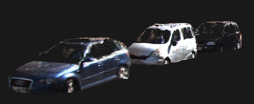
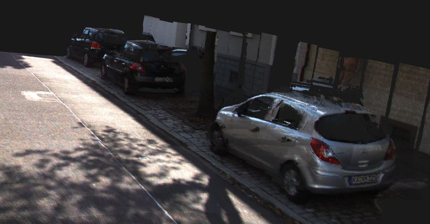
B. Map and Texture Analysis
   Labeled Ground truth for textured maps doesn’t exist;
hence, we project the LIDAR points into the camera and
generate ground truth for the color texture. Later, we compare
the generated textured map against the accurate 3D data
provided by the LIDAR and the generated color texture
ground truth. In order to have a fair comparison, we manually
remove moving object points both from ground truth and the
                                                                                                            (a)
textured map by using publicly available tool CloudCompare
[41]. Moreover, We set the foveal regions to
                  0m ≤ near blind zone < 3m,
                  3m ≤ white zone < 15m,
                 15m ≤ f ar blind zone
   In Table II, we have shown M E, T E and M T M E for
the textured maps generated using proposed framework
and those generated using baselines4 . We also compare
                                                                                                            (b)
M E for seq 0095 with [21], [24]. For this we rely only
on their results provided in the paper due to unavailability
of their code. As the previous works, [24], [21], [42]
are bound to produce only qualitative analysis of their
texturing process, we compare our results for T E and
M T M E against the baselines. The best and the worst
results of proposed and baselines are shown in blue and red.

   1) Map Error: For the seq. 0095, the proposed
framework achieves the best µM E of 0.010m in E6                                                            (c)
and outperforms [21] by 88%, [24] by 87% as well as                          Fig. 9: Zoom in for better insight. Figure (a), (b) close up
the baselines GEN-ICP by 90%, STD-ICP by 99%, and                            of the generated textured maps for sequence 0095, and (c)
P2P-ICP by 99%. While for the seq. 0001, the proposed                        sequence 0001.
framework achieves best µM E of 0.008m in E4. For
this sequence, all of the E4-E7 have almost similar µM E
which is not the case with seq. 0095. It indicates that
                                                                             9. It should be noted that T E also captures the effect of
pose-refinement is dependent on the 3D information
                                                                             oversampling as seen in E3, E7 and E11, especially in the
in LIDAR scans. Its effect is also indicated by µM E for seq
                                                                             seq 0095.
0095 as GEN-ICP in E3 is trapped in local minima due to
oversampling.
                                                                                3) Mean Texture Mapping Error: In order to asses the
                                                                             overall performance of the algorithm, we also report
   2) Texture Error: Here, we claim that M E doesn’t con-
                                                                             M T M E (Eq. 5) for all of our experiments. From the table
vey any details about the texture quality of the map. It is
                                                                             II, especially from the baseline experiments, it can be seen
indicated by large T E in all of the baselines GEN-ICP,
                                                                             that M T M E is high when either of M E or T E is high and
STD-ICP, P2P-ICP (Table II). All of the baselines show µT E
                                                                             attains lower values only when both of the M E and T E are
greater than 140 which is ∼ 54% of the maximum attainable
                                                                             lower. From the table II, it can also be noticed that incorpora-
value 255 for each of the red, green, blue component of a
                                                                             tion of ray-filtering reduces the M T M E drastically.
pixel color. This large error shows the usefulness of Eq. 4.
                                                                             For seq 0095, E2 outperforms it’s baseline version GEN-
   For both of the sequence, the proposed ray-filtering
                                                                             ICP by 95%, E6 outperforms STD-ICP by 98% and E10
+ foveal-processing technique drastically reduces
                                                                             outperforms P2P-ICP by 98%. Similarly, for seq 0001, all
the T E. It is evident from the µT E of E0-E11. The best
                                                                             the three of E0-E11 outperforms their baselines by more
achieved µT E for 0095, 0001 is 8.328 and 5.24 respectively
                                                                             than 95%. These visible effects of the reduced M T M E are
which are only ∼ 3% and 2% of the maximum value
                                                                             shown in fig. 9.
(255). These values of µT E are far superior to the best
145.85 of the baselines without ray-filtering +                                                    V. C ONCLUSION
foveal-processing. Effect of these improved T E is
                                                                                In this paper we presented robust framework to gener-
clearly visible by realistic texture transfer as shown in fig.
                                                                             ate high quality textured 3D maps of urban areas. While
  4 align the scans, obtain color texture by projecting LIDAR point to the   development of this framework, we have focused on three
camera and accumulate in a local frame L                                     major tasks: (i) incremental accurate scan alignment, (ii) real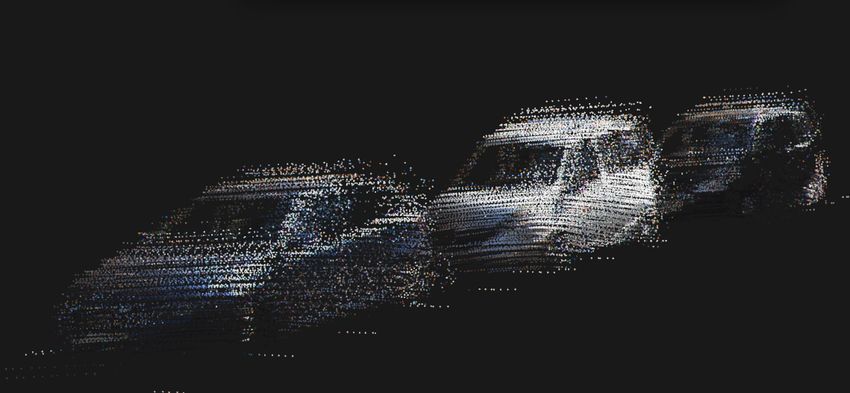
·10−2 ·102
Average Error (m) 15 GEN-ICP GEN-ICP GEN-ICP GEN-ICP
Map Error (m)
1
Texture Error
STD-ICP 3 STD-ICP STD-ICP 150 STD-ICP
Time (sec)
P2P-ICP P2P-ICP P2P-ICP P2P-ICP
10 2 100
0.5
1 50
5
0 0 0
Baseline 0xUp 1xUp 2xUp 3xUp baseline 0xUp 1xUp 2xUp 3xUp baseline 0xUp 1xUp 2xUp 3xUp baseline 0xUp 1xUp 2xUp 3xUp
·10−2 ·102 ·10−2
Average Error (m)
14 GEN-ICP GEN-ICP GEN-ICP 150 GEN-ICP
Map Error (m)
1
Texture Error
STD-ICP STD-ICP STD-ICP STD-ICP
Time (sec)
P2P-ICP P2P-ICP P2P-ICP P2P-ICP
12 4
100
10 0.5
2 50
8
0 0
baseline 0xUp 1xUp 2xUp 3xUp baseline 0xUp 1xUp 2xUp 3xUp baseline 0xUp 1xUp 2xUp 3xUp baseline 0xUp 1xUp 2xUp 3xUp
(a) Scan matching analysis (b) Timing performance (c) Mapping error (d) Texture quality
Fig. 10: Performance Analysis of the framework. Columns (a) scan matching performance analysis, (b) Timing analysis
while scan matching, (c) µM E of map error, and (d) µT E of texture error. The first and second row corresponds to the
sequence 0095 and 0001 respectively.
TABLE II:
Quantitative evaluation of the proposed framework and various baselines. Here, “pose-r”, “ray-f”, “fov-p” stands for
pose-refinement, ray-filtering and foveal-processing respectively.
KITTI Seq 0095 KITTI Seq 0001
Algorithm
M E (m) TE M E (m) TE
MT ME MT ME
µM E σM E µT E σT E µM E σM E µT E σT E
[21] 0.089 0.131 – – – – – – – –
[24] 0.082 0.098 – – – – – – – –
baseline GEN-ICP 0.102 0.089 158.51 117.50 12.648 0.052 0.064 152.66 90.51 7.744
pose-r (GEN-ICP) + 0xUp + ray-f + fov-p (E0) 0.098 0.089 57.42 74.60 6.899 0.014 0.045 6.49 22.97 0.098
pose-r (GEN-ICP) + 1xUp + ray-f + fov-p (E1) 0.050 0.081 31.65 70.83 2.300 0.014 0.044 6.37 22.61 0.094
pose-r (GEN-ICP) + 2xUp + ray-f + fov-p (E2) 0.036 0.075 28.39 70.01 0.513 0.014 0.045 6.13 21.93 0.095
pose-r (GEN-ICP) + 3xUp + ray-f + fov-p (E3) 0.104 0.095 58.78 87.81 7.643 0.014 0.045 6.11 21.62 0.092
baseline STD-ICP 1.076 3.077 174.42 117.85 16.229 0.033 0.046 145.85 90.93 4.835
pose-r (STD-ICP) + 0xUp + ray-f + fov-p (E4) 0.066 0.085 45.10 77.41 6.133 0.008 0.033 6.80 24.03 0.062
pose-r (STD-ICP) + 1xUp + ray-f + fov-p (E5) 0.010 0.040 13.17 49.44 0.286 0.009 0.032 6.77 23.38 0.064
pose-r (STD-ICP) + 2xUp + ray-f + fov-p (E6) 0.010 0.042 8.328 36.79 0.268 0.012 0.041 6.27 22.35 0.078
pose-r (STD-ICP) + 3xUp + ray-f + fov-p (E7) 0.030 0.069 19.88 57.22 2.501 0.013 0.044 5.24 20.36 0.069
baseline P2P-ICP 1.086 3.084 170.32 114.47 15.814 0.037 0.055 155.76 90.17 5.759
pose-r (P2P-ICP) + 0xUp + ray-f + fov-p (E8) 0.092 0.091 54.02 71.12 7.687 0.010 0.038 7.88 29.14 0.087
pose-r (P2P-ICP) + 1xUp + ray-f + fov-p (E9) 0.037 0.067 16.64 56.91 0.236 0.012 0.041 7.32 27.28 0.092
pose-r (P2P-ICP) + 2xUp + ray-f + fov-p (E10) 0.021 0.051 12.59 46.72 0.201 0.013 0.045 6.25 23.59 0.092
pose-r (P2P-ICP) + 3xUp + ray-f + fov-p (E11) 0.040 0.080 20.96 58.16 2.775 0.014 0.047 5.78 22.07 0.088
time dense upsampling of 3D scans and (iii) color texture www.velodyne.com/lidar/products/white paper.
transfer without loosing fine grained details. The proposed [2] Ladybug3, “Spherical vision products: Ladybug3,” tech. rep., Point-
grey, 2009. Specification sheet and documentations available at
framework successfully accomplishes all of the above three www.ptgrey.com/products/ladybug3/index.asp.
tasks by collectively leveraging multimodal information i.e. [3] F. Chabot, M. Chaouch, J. Rabarisoa, C. Teulière, and T. Chateau,
LIDAR scans, images, navigation data. The generated maps “Deep MANTA: A coarse-to-fine many-task network for joint
by using this framework, appears significantly realistic and 2d and 3d vehicle analysis from monocular image,” CoRR,
vol. abs/1703.07570, 2017.
carries fine grained details both in terms of 3D surface and [4] X. Chen, K. Kundu, Z. Zhang, H. Ma, S. Fidler, and R. Urtasun,
color texture. Such high quality textured 3D maps can be “Monocular 3d object detection for autonomous driving,” in Pro-
used in several applications including precise localization of ceedings of the IEEE Conference on Computer Vision and Pattern
Recognition, pp. 2147–2156, 2016.
the vehicle, it can be used as a virtual 3D environment for [5] S. Ren, K. He, R. Girshick, and J. Sun, “Faster r-cnn: Towards real-
testing various algorithms related to autonomous navigation time object detection with region proposal networks,” in Advances in
without deploying the algorithm on a real vehicle and it can neural information processing systems, pp. 91–99, 2015.
also be used as background map in computer games for real [6] K. He, G. Gkioxari, P. Dollár, and R. B. Girshick, “Mask r-cnn,” 2017
IEEE International Conference on Computer Vision (ICCV), pp. 2980–
life gaming experience. 2988, 2017.
[7] H. Zhao, J. Shi, X. Qi, X. Wang, and J. Jia, “Pyramid scene parsing
R EFERENCES network,” in Proceedings of IEEE Conference on Computer Vision and
[1] Velodyne, “Velodyne HDL-64E: A high definition LIDAR sensor for Pattern Recognition (CVPR), 2017.
3D applications,” tech. rep., Velodyne, October 2007. Available at [8] M. Buehler, K. Iagnemma, and S. Singh, The DARPA urban challenge:
autonomous vehicles in city traffic, vol. 56. springer, 2009.             [32] Q. Pan, G. Reitmayr, and T. Drummond, “Proforma: Probabilistic
 [9] D. Lavrinc, “Ford unveils its first autonomous vehicle pro-                    feature-based on-line rapid model acquisition.,” in BMVC, vol. 2, p. 6,
     totype http://www. wired. com/autopia/2013/12/ford-fusion-hybrid-              Citeseer, 2009.
     autonomous,” Accessed December 16th, 2013.                                [33] V. Litvinov and M. Lhuillier, “Incremental solid modeling from sparse
[10] E. Ackerman, “Tesla model S: Summer software update will enable                and omnidirectional structure-from-motion data,” in British Machine
     autonomous driving,” IEEE Spectrum Cars That Think, 2015.                      Vision Conference, 2013.
[11] R. W. Wolcott and R. M. Eustice, “Fast lidar localization using           [34] D. I. Lovi, “Incremental free-space carving for real-time 3d recon-
     multiresolution gaussian mixture maps,” in Proceedings of the IEEE             struction,” 2011.
     International Conference on Robotics and Automation, pp. 2814–2821,       [35] V. Litvinov and M. Lhuillier, “Incremental solid modeling from sparse
     May 2015.                                                                      structure-from-motion data with improved visual artifacts removal,” in
[12] J. Levinson and S. Thrun, “Robust vehicle localization in urban                Pattern Recognition (ICPR), 2014 22nd International Conference on,
     environments using probabilistic maps,” in Proceedings of the IEEE             pp. 2745–2750, IEEE, 2014.
     International Conference on Robotics and Automation, 2010.                [36] G. Harary, A. Tal, and E. Grinspun, “Context-based coherent surface
[13] T. Wu and A. Ranganathan, “Vehicle localization using road mark-               completion,” ACM Transactions on Graphics (TOG), vol. 33, no. 1,
     ings,” in Intelligent Vehicles Symposium (IV), 2013 IEEE, pp. 1185–            p. 5, 2014.
     1190, June 2013.                                                          [37] M. A. Fischler and R. C. Bolles, “Random sample consensus: a
[14] S. Sukkarieh, E. M. Nebot, and H. F. Durrant-Whyte, “A high integrity          paradigm for model fitting with applications to image analysis and
     imu/gps navigation loop for autonomous land vehicle applications,”             automated cartography,” in Readings in computer vision, pp. 726–740,
     IEEE Transactions on Robotics and Automation, vol. 15, no. 3,                  Elsevier, 1987.
     pp. 572–578, 1999.                                                        [38] R. DeVoe, H. Ripps, and H. Vaughan, “Cortical responses to stimu-
[15] B. Barshan and H. F. Durrant-Whyte, “Inertial navigation systems               lation of the human fovea,” Vision Research, vol. 8, no. 2, pp. 135 –
     for mobile robots,” IEEE Transactions on Robotics and Automation,              147, 1968.
     vol. 11, no. 3, pp. 328–342, 1995.                                        [39] M. Callieri, P. Cignoni, M. Corsini, and R. Scopigno, “Masked photo
[16] J. Folkesson and H. Christensen, “Graphical SLAM—A self-correcting             blending: Mapping dense photographic data set on high-resolution
     map,” in Proceedings of the IEEE International Conference on                   sampled 3d models,” Computers & Graphics, vol. 32, no. 4, pp. 464–
     Robotics and Automation, pp. 383–390, 2004.                                    473, 2008.
[17] E. Olson, J. Leonard, and S. Teller, “Fast iterative alignment of pose    [40] A. Geiger, P. Lenz, C. Stiller, and R. Urtasun, “Vision meets robotics:
     graphs with poor estimates,” in Proceedings of the IEEE International          The kitti dataset,” The International Journal of Robotics Research,
     Conference on Robotics and Automation, pp. 2262–2269, 2006.                    vol. 32, no. 11, pp. 1231–1237, 2013.
[18] R. M. Eustice, H. Singh, and J. J. Leonard, “Exactly sparse delayed-      [41] D. Girardeau-Montaut, “Cloud compare—3d point cloud and mesh
     state filters for view-based SLAM,” IEEE Transactions on Robotics,             processing software,” Open Source Project, 2015.
     vol. 22, no. 6, pp. 1100–1114, 2006.                                      [42] K. Yousif, A. Bab-Hadiashar, and R. Hoseinnezhad, “Real-time rgb-
[19] H. Durrant-Whyte, N. Roy, and P. Abbeel, “A linear approximation for           d registration and mapping in texture-less environments using ranked
     graph-based simultaneous localization and mapping,” in Proceedings             order statistics,” in Intelligent Robots and Systems (IROS 2014), 2014
     of Robotics: Science and Systems, pp. 41–48, MIT Press, 2012.                  IEEE/RSJ International Conference on, pp. 2654–2660, IEEE, 2014.
[20] G. Grisetti, R. Kuemmerle, C. Stachniss, and W. Burgard, “A tutorial
     on graph-based SLAM,” Intelligent Transportation Systems Magazine,
     IEEE, vol. 2, no. 4, pp. 31–43, 2010.
[21] A. Romanoni and M. Matteucci, “Incremental reconstruction of urban
     environments by edge-points delaunay triangulation,” in Intelligent
     Robots and Systems (IROS), 2015 IEEE/RSJ International Conference
     on, pp. 4473–4479, IEEE, 2015.
[22] N. Engelhard, F. Endres, J. Hess, J. Sturm, and W. Burgard, “Real-time
     3d visual slam with a hand-held rgb-d camera,” in Proc. of the RGB-
     D Workshop on 3D Perception in Robotics at the European Robotics
     Forum, Vasteras, Sweden, vol. 180, pp. 1–15, 2011.
[23] B. Triggs, P. F. McLauchlan, R. I. Hartley, and A. W. Fitzgibbon,
     “Bundle adjustment—a modern synthesis,” in International workshop
     on vision algorithms, pp. 298–372, Springer, 1999.
[24] A. Romanoni, D. Fiorenti, and M. Matteucci, “Mesh-based 3d tex-
     tured urban mapping,” 2017 IEEE/RSJ International Conference on
     Intelligent Robots and Systems (IROS), pp. 3460–3466, 2017.
[25] P. J. Besl and N. D. McKay, “Method for registration of 3-d shapes,” in
     Sensor Fusion IV: Control Paradigms and Data Structures, vol. 1611,
     pp. 586–607, International Society for Optics and Photonics, 1992.
[26] R. Bergevin, M. Soucy, H. Gagnon, and D. Laurendeau, “Towards
     a general multi-view registration technique,” IEEE Transactions on
     Pattern Analysis and Machine Intelligence, vol. 18, no. 5, pp. 540–
     547, 1996.
[27] A. Segal, D. Haehnel, and S. Thrun, “Generalized-icp.,” in Robotics:
     science and systems, vol. 2, 2009.
[28] M. Alexa, J. Behr, D. Cohen-Or, S. Fleishman, D. Levin, and C. T.
     Silva, “Computing and rendering point set surfaces,” IEEE Transac-
     tions on visualization and computer graphics, vol. 9, no. 1, pp. 3–15,
     2003.
[29] S. Gould, J. Arfvidsson, A. Kaehler, B. Sapp, M. Messner, G. R.
     Bradski, P. Baumstarck, S. Chung, A. Y. Ng, et al., “Peripheral-foveal
     vision for real-time object recognition and tracking in video.,” in
     IJCAI, vol. 7, pp. 2115–2121, 2007.
[30] J. Ba, V. Mnih, and K. Kavukcuoglu, “Multiple object recognition
     with visual attention,” arXiv preprint arXiv:1412.7755, 2014.
[31] A. Ablavatski, S. Lu, and J. Cai, “Enriched deep recurrent visual
     attention model for multiple object recognition,” in Applications of
     Computer Vision (WACV), 2017 IEEE Winter Conference on, pp. 971–
     978, IEEE, 2017.
You can also read