APPENDIX D
HYDRAULIC MODEL DEVELOPMENT
←
→
Page content transcription
If your browser does not render page correctly, please read the page content below
APPENDIX D HYDRAULIC MODEL DEVELOPMENT
THIS PAGE INTENTIONALLY LEFT BLANK
DOSEWALLIPS RESILIENCY PLAN: HYDRAULIC MODEL
DEVELOPMENT APPENDIX
HYDRAULIC MODEL DEVELOPMENT
A hydraulic model of the Dosewallips River was developed using Hydronia’s RiverFlow-2D Plus GPU and Aquaveo
SMS v13.0 computer software. RiverFlow-2D is a two-dimensional finite volume computer model that provides
depth averaged hydraulic parameters at centroids within a triangular mesh model domain.

Mesh Development and Roughness Categories
The model domain encompasses 2 river miles, with the upper boundaries just upstream of river mile (RM) 3, and
the lower boundary at RM 1 where the floodplain narrows into a bedrock canyon. The topographic data is from
LiDAR collected in 2017/2018 (Quantum Spatial, 2019).
The model mesh was created with fine mesh spacing in the channel and in floodplain channels, with expanded
mesh spacing in less topographically complex areas further from the stream, using criteria for mesh spacing
shown in Table 1.
Table 1. Mesh Spacing Guidelines for Breakline Categories
            LOCATION                                VERTEX SPACING (FT)
 Road                                                                                          10
 Bank                                                                                          10
 Floodplain channels                                                                           10
 Boundary                                                                                      15

Hydraulic resistance is characterized in the model by polygons representing differing surface roughness types
such as main channel, pasture, or paved road. The full list of roughness categories and their associated
Manning’s n values is in Table 3. Roughness categories were manually delineated using 2017 aerial imagery.
Table 2. Calibrated Manning's n roughness values for each roughness category.
            CATEGORY                                  MANNING'S N VALUE
 Active Channel                                                                             0.035
 Side Channel                                                                               0.045
 Forested Gravel Bar                                                                         0.08
 Bare Earth                                                                                  0.03
 Pasture                                                                                     0.03
 Forest                                                                                      0.08
 Road                                                                                       0.015
 Natural Logjam                                                                              0.15
 Building                                                                                    0.99

                                                                                                                1
NATURAL SYSTEMS DESIGN | April 28, 2021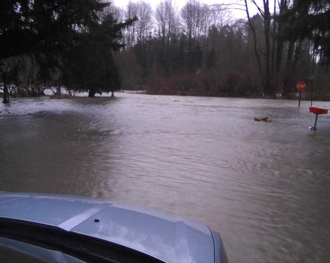
JEFFERSON COUNTY PUBLIC HEALTH DEPARTMENT DOSEWALLIPS POWERLINES/LAZY C RESILIENCY PLAN – HYDRAULIC MODEL DEVELOPMENT APPENDIX
Hydrology and Model Boundary Conditions
The model was run for a series of three representative flow scenarios – the 1-year, 10-year, and 100-year floods
– to evaluate hydraulic parameters at the project site. To develop estimated inflows for the Dosewallips model,
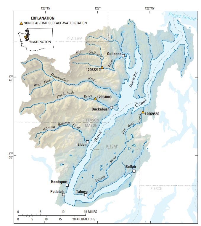
NSD performed a hydrologic analysis of the region. This analysis focused on two USGS gages: USGS gage
#12053000, Dosewallips River near Brinnon, WA (henceforth referred to as the Dosewallips gage) and USGS
gage #120454000, Duckabush River near Brinnon, WA (henceforth the Duckabush gage) (Figure 1). Accurately
representing the magnitude of peak flows within the project reach is challenging because the Dosewallips gage
only operated from 1930-1951, and so offers only a small and out-of-date period of record from which to
extrapolate. No other gage with a greater period of record was available on the Dosewallips River. To account
for this, the Duckabush gage was identified as a possible surrogate to streamflow conditions on the Dosewallips
River. The Duckabush River watershed is south of and directly adjacent to the Dosewallips River watershed and
has similar characteristics of slope, relief, precipitation, and land use (Table 3).
12053000
Figure 1. Map of Dosewallips and Duckabush Basins showing locations of USGS gages.
2
NATURAL SYSTEMS DESIGN | April 28, 2021JEFFERSON COUNTY PUBLIC HEALTH DEPARTMENT DOSEWALLIPS POWERLINES/LAZY C RESILIENCY PLAN – HYDRAULIC MODEL DEVELOPMENT APPENDIX
Table 3 Basin characteristics for the Dosewallips and Duckabush Rivers. Data downloaded from Stream
Stats (USGS 2016).
Parameter Dosewallips River Dosewallips River at Duckabush River at
at USGS Gage Lazy C USGS Gage
Drainage Area (mi2) 93 113 66
Basin average annual
96 90 110
precipitation (in)
Mean basin slope (%) 62% 60% 63%
Canopy Cover (%) 60% 63% 65%
Mean basin elevation (ft) 4140 3740 3530
Maximum basin elevation (ft) 7770 7770 6750
Minimum basin elevation (ft) 306 65 271
Relief (ft) 7460 7700 6480
To estimate discharge values on the mainstem, a peak flow analysis of both the Dosewallips gage and the
Duckabush gage was performed using Log-Pearson schedule 3b methodology. For the Dosewallips gage, the
resulting 10-year and 100-year flows were then scaled to the project site using the USGS drainage-area ratio
method for ungaged sites, which involves a weighted average of the USGS regional regression equation results
with the drainage-area-scaled results of the gage analysis. For the Duckabush gage, since the drainage area ratio
of the ungaged site to the gage was over 1.5, the USGS regional regression equation results and the drainage-
area-scaled results of the gage analysis were given equal weight and the reported 10-year and 100-year results
are a simple average of the two. The 1-year flow was scaled from each gage using a simple drainage area ratio,
as the USGS does not provide coefficients for its regional regression equations for this recurrence interval.
To identify discharge estimates for each recurrence interval, the results of the above analysis of the Duckabush
and Dosewallips were compared. Since the Duckabush gage has a greater and more current period of record,
the 10-year and 100-year floods scaled from the Duckabush gage were used as the estimated discharge values
for the hydraulic model. The 1-year flood used for the hydraulic model is an average of the discharge value
scaled from the Duckabush and the Dosewallips gage, since there was no USGS regional regression equation
available for this recurrence interval and therefore the estimates are less certain. Table 4 shows the scaled
results of the gage analyses as well as the final estimated discharge values for the project site.
The hydraulic model was built using 2019 LiDAR that was collected on on 10/6/17 and 7/22/18 and does not
contain bathymetry data. Average discharge on these days was 50 cfs and 140 cfs on the Duckabush gage
respectively. Since it is unknown which day the project area was captured, 50 cfs was adopted as the LiDAR flow
to be conservative. This flow was determined to be low enough in comparison to the scale of the flood flows
being modeled that it would not affect the results. Therefore since the models are run on top of a water surface
that corresponds to a discharge of 50 cfs, 50 cfs was subtracted from each of the discharge values shown in
Table 4 to arrive at the final model inflow values.
The models were run in a simulated steady state; i.e., the inflow hydrographs look like stair steps, with each
peak flow of interest running long enough for the model to equilibrate before jumping to the next flow of
interest. The model has only one outflow boundary, which was set to uniform flow outflow with a slope of
0.0003 ft/ft.
3
NATURAL SYSTEMS DESIGN | April 28, 2021JEFFERSON COUNTY PUBLIC HEALTH DEPARTMENT DOSEWALLIPS POWERLINES/LAZY C RESILIENCY PLAN – HYDRAULIC MODEL DEVELOPMENT APPENDIX
Table 4. Estimated Discharge Values
RECURRENCE DISCHARGE AT PROJECT DISCHARGE AT FINAL DISCHARGE
INTERVAL SITE SCALED FROM PROJECT SITE SCALED ESTIMATE AT
DOSEWALLIPS GAGE FROM DUCKABUSH PROJECT SITE
(CFS) GAGE (CFS) (CFS)
1-year 1,620 2,570 2,100
10-year 9,180 11,420 11,420
100-year 15,900 17,120 17,120
Climate Change Estimates
Once peak flows were determined for the project site, it was necessary to estimate the impact that climate
change would have on these flows in order to understand and model future floods. The Columbia Basin Climate
Change Scenarios (CBCCS) project summarizes climate change projections for many watersheds, the closest to
the Dosewallips being the Skokomish River (Hamlet 2010). For each basin the CBCCS projects the 20-year, 50-
year, and 100-year recurrence interval floods into the future to estimate their magnitude in the years 2070-2099
based on one of two climate change scenarios. For this project the A1B climate change scenario was used, which
is the higher of the two scenarios and the closest to current climate change projections.
Data were downloaded from the Columbia Basin Climate Change Scenarios Project website at
http://warm.atmos.washington.edu/2860/. These materials were produced by the Climate Impacts Group at the
University of Washington in collaboration with the WA State Department of Ecology, Bonneville Power
Administration, Northwest Power and Conservation Council, Oregon Water Resources Department, and the B.C.
Ministry of the Environment. The percent change in the Skokomish River floods from 2020 to 2070-2099 as
estimated by the CBCCS was determined and then applied as a multiplier to the Dosewallips floods to estimate
climate change flows (Table 5). Note that the lowest flood for which the CBCCS makes estimates is the 20-year
flood; therefore, the multiplier applied to the Dosewallips 1-year and 10-year floods is the CBCCS-estimated 20-
year flood percent increase. These are likely conservative estimates as the relative impact of climate change
would be expected to decrease with the frequency of the flood.
Table 5. The magnitude of future peak flows projected with climate change impacts for 2070-2099.
RECURRENCE PRESENT DISCHARGE PERCENT INCREASE DUE FUTURE (2070-2099)
INTERVAL ESTIMATE AT LAZY C TO CLIMATE CHANGE DISCHARGE
(CFS) ESTIMATE AT LAZY C
(CFS)
1-year 2,100 18% 2,480
10-year 11,420 18% 13,480
100-year 17,120 23% 21,060
Validation
To ensure that the model accurately reflects real world conditions, data provided by the community regarding
locations, depths, and timings of flooding was compared to model results.
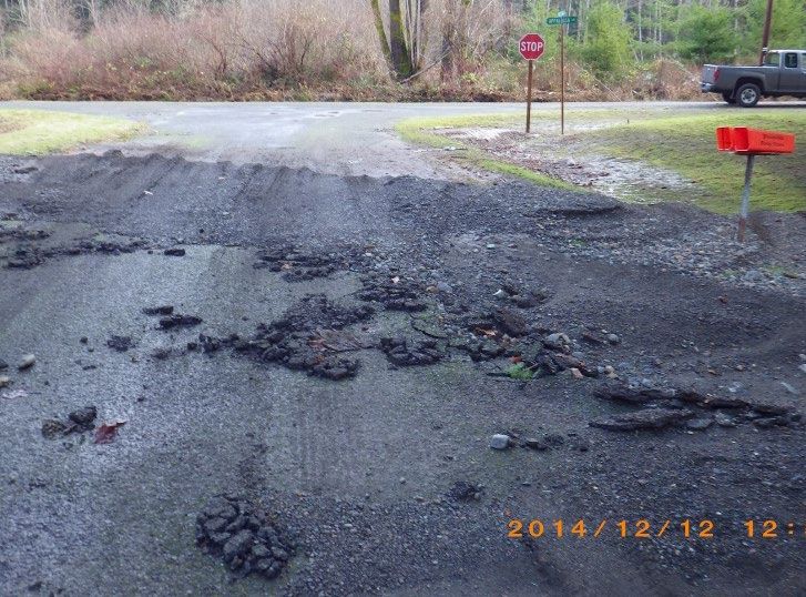
The first point of comparison was provided by a picture taken of flooding on the intersection of Appaloosa Dr
and Mustang Lane on December 11, 2014 at 10:40 am, and a picture of the same location the following day after
the flood had receded (Figure 2). By comparing the stop sign in the two pictures, it is possible to estimate that
the depth of water during flooding in the location was approximately 2 ft. Flow at the Duckabush gage at this
date and time was around 2,500 cfs, which tells us that flow at the project site was approximately 4,200 cfs
when the flow is scaled by drainage area. The magnitude of this flow falls in between the modeled 1-year and
4
NATURAL SYSTEMS DESIGN | April 28, 2021JEFFERSON COUNTY PUBLIC HEALTH DEPARTMENT DOSEWALLIPS POWERLINES/LAZY C RESILIENCY PLAN – HYDRAULIC MODEL DEVELOPMENT APPENDIX
10-year recurrence intervals floods; however, the model has a brief ramp-up period in which discharge increases
from the 1-year magnitude to the 10-year magnitude during which results at intermediate flows can be seen. At
the 1-year flood, when discharge is 2,100 cfs, this intersection is not inundated, and at the 10-year flood when
discharge is 11,420 cfs, this intersection is under 0.5-2.5 ft of water. Intermediate results are less reliable as the
model is not given time to equilibrate at intermediate flows, but the model shows that this intersection begins
to partially inundate when mainstem flow is approximately 4,300 cfs, at which point the depth is up to 1.8 ft,
and is fully inundated when mainstem flow reaches approximately 6,700 cfs.
Given the uncertainties surrounding flow estimates on the day of the photo (since the estimate must be based
on a different basin, see Hydrology section), as well as the approximate nature of the depth estimate from the
photo, an exact match from the model should not be expected. This photo therefore validates the model – both
show inundation of approximately 2 ft at this intersection when flow is between 4,000 cfs and 4,500 cfs. The
model does not show full inundation of the intersection until 6,700 cfs , while the photo shows full inundation at
what was estimated to be 4,200 cfs, but as mentioned above the intermediate results between the 1-year and
10-year floods are not given time to equilibrate in the model so this discrepancy may simply be a result of the
model being focused on different flood sizes.
Figure 2. Picture of 2014 flooding at the intersection of Appaloosa Dr and Mustang Ln (left) compared to a
picture of the same intersection the following day (right).
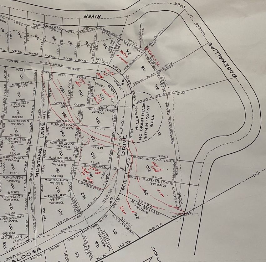
The second point of comparison is a parcel map marked up by landowners to illustrate the flow path that floods
typically take through the Lacy C development based on their experience (Figure 3). This is not associated with
any particular discharge or depth but can be compared to the flowpath that the model shows floodwaters
following when they first enter the Lazy C development. Figure 4 shows the model results in the same area at
approximately 5,400 cfs, as floodwaters are just entering the Lazy C development. The flowpath in Figure 4
mirrors that drawn by landowners in Figure 3 – the crossing of Appaloosa Dr is at the same place, and
floodwaters come up through parcels 29 and 30 in the model as drawn. Between Appaloosa Drive and Mustang
Lane there is some deviation due to the complexity of topography, but the general pattern of flow from parcel
159 to the intersection of Appaloosa Dr and Mustang Lane is the same.
5
NATURAL SYSTEMS DESIGN | April 28, 2021JEFFERSON COUNTY PUBLIC HEALTH DEPARTMENT DOSEWALLIPS POWERLINES/LAZY C RESILIENCY PLAN – HYDRAULIC MODEL DEVELOPMENT APPENDIX
Figure 3. Parcel map marked up by landowners in red to illustrate typically flood flow path.
Figure 4. Hydraulic model results at approximately 5,400 cfs overlaid on the parcel map, showing the flow
path of floodwaters as they enter the Lazy C development.
6
NATURAL SYSTEMS DESIGN | April 28, 2021JEFFERSON COUNTY PUBLIC HEALTH DEPARTMENT DOSEWALLIPS POWERLINES/LAZY C RESILIENCY PLAN – HYDRAULIC MODEL DEVELOPMENT APPENDIX
REFERENCES
Hamlet, A.F., P. Carrasco, J. Deems, M.M. Elsner, T. Kamstra, C. Lee, S-Y Lee, G. Mauger, E. P. Salathe, I. Tohver,
L. Whitely Binder, 2010, Final Project Report for the Columbia Basin Climate Change Scenarios Project,
http://warm.atmos.washington.edu/2860/report/.
Mastin, M.C., Konrad, C.P., Veilleux, A.G., and Tecca, A.E., 2016, Magnitude, frequency, and trends of floods at
gaged and ungaged sites in Washington, based on data through water year 2014 (ver 1.2, November
2017): U.S. Geological Survey Scientific Investigations Report 2016–5118, 70 p.,
http://dx.doi.org/10.3133/sir20165118.
Quantum Spatial, 2019. Olympic Peninsula, Washington 3DEP Lidar – Area 1 Technical Data Report. Project
conducted on behalf of the U.S. Geological Survey.
U.S. Geological Survey, 2016, The StreamStats program, online at http://streamstats.usgs.gov, accessed on
2/14/2021.
7
NATURAL SYSTEMS DESIGN | April 28, 2021You can also read