Application Checkpoint and Power Study on Large Scale Systems
←
→
Page content transcription
If your browser does not render page correctly, please read the page content below

Application Checkpoint and Power Study on Large Scale
                                                                   Systems
                                                                                           Yuping Fan†
                                                                              †
                                                                                  Illinois Institute of Technology

                                                                                          ABSTRACT
                                        Power efficiency is critical in high performance computing (HPC) systems. To achieve high power efficiency on
                                        application level, it is vital importance to efficiently distribute power used by application checkpoints. In this
                                        study, we analyze the relation of application checkpoints and their power consumption. The observations could
arXiv:2109.01943v1 [cs.SE] 4 Sep 2021

                                        guide the design of power management.
                                        Keywords: High Performance Computing (HPC), power management, performance analysis

                                                                                     1. INTRODUCTION
                                        As the size of HPC systems rapidly increasing, the amount of electrical power consumed by HPC systems are
                                        keeping increasing. As a result, power becomes the leading constraint for the design of the next generation HPC
                                        systems. There are several existing solutions, such as power capping and dynamic voltage and frequency scaling
                                        (DVFS), to address the power constraints. To efficient distribute power, it is crucial to analyze application
                                        behaviors and provide customized power policies for various applications.
                                           Checkpointing is the widely used fault tolerate mechanism. Checkpoints can be categorized into system-level
                                        and application-level checkpoints. Application-level checkpoints aim to recover failed applications. Applications
                                        can choose their own checkpoint frequency and other parameters related to checkpoints.
                                            Power and time consumed by checkpointing is not negligible. Therefore, this work studies how the checkpoint
                                        and faults affect the power and energy consumption. We utilize the MonEQ1 to gather the power information
                                        on Mira. MonEQ is a user-level profiling library, which collects power information at node card level. Beside the
                                        node card power information as a whole, the power information breaks down into six domains, which are dram
                                        voltage, link chip voltage, SRAM voltage, optics voltage, optics voltage, PCIExpress voltage and link chip core
                                        voltage. Three benchmarks, NPB,2 Flash3 and Stream,4 are investigated in this study. For NPB and Stream
                                        benchmarks, we add the checkpoints and faults by FTI.5 FTI is a fault tolerance interface, which provides
                                        application level checkpointing for large-scale supercomputers. Four configurable checkpoint levels are offered in
                                        FTI, which provides different levels of protection for applications. The checkpoint frequencies can be configured
                                        and be optimized6 to achieve the balance between execution time and program correctness. Flash benchmark
                                        has its own checkpointing strategy, but there is no option to inject faults.
                                           The observations in this study can guide HPC job scheduler to intelligently schedule jobs7–17 and wisely set
                                        checkpoint strategies in order to achieve high power efficiency.
                                            The remainder of this paper is organized as follows. We start by introducing background and related work
                                        in §2. §3 presents the analysis and observation. We conclude the paper in §4.

                                                                                      2. BACKGROUND
                                        This section introduces HPC power management in §2.1 and Application Checkpointing §2.2. Then, we introduce
                                        the benchmarks analyzed in this study (§2.3).
2.1 HPC Power Management
As the size of HPC systems size rapidly grow, the limited power budget becomes one of the most crucial
challenges. Several hardward power management mechanisms, such as dynamic voltage and frequency scaling
(DVFS) and power capping, have been developed. Power can be management either at the system level or at
the application level. Studies show that managing power at application level is more efficient. This is because
the effects of power capping on different applications vary. Even the effects of power capping on different stages
of an applications vary. Therefore, to efficient manage power, it is crucial to comprehensively analyze the effects
of power management on individual applications.

2.2 Application Checkpointing
Fault tolerance is a serious problem in HPC systems. HPC systems consist of millions of components. A single
point of failure could lead to application failure, or even system failure. As the HPC system sizes rapidly
increasing, the failures are happened more frequently. Checkpointing is one of the most widely used fault
tolerance techniques. HPC checkpointing can be implemented in two levels: system level and application level.
System level checkpointing can prevent catastrophic system failures, but it is very time- and memory- intensive.
On the other hand, application checkpointing is more lightweight and can prevent application failures. Typically,
application checkpointing is scheduled more often than system checkpointing.

2.3 Benchmarks
In order to comprehensively evaluate various types of applications performance, three benchmarks are studied
in this work.

2.3.1 NPB benchmarks
The NAS Parallel Benchmarks (NPB) are a small set of programs designed to help evaluate the performance
of highly parallel supercomputers. The benchmarks are derived from computational fluid dynamics (CFD)
applications and consist of five kernels and three pseudo-applications. We study three representative programs
from NPB benchmarks:

  1. CG: Conjugate Gradient, irregular memory access and communication
  2. FT: discrete 3D fast Fourier Transform, all-to-all communication

  3. LU: Lower-Upper Gauss-Seidel solver

2.3.2 Flash
Flash benchmark is multiphysics multiscale simulation code. We select Sedov explosion problem in this study.
The Sedov explosion problem is a hydrodynamical test to check the code’s ability to deal with strong shocks and
non-planar symmetry.

2.3.3 STREAM
STREAM is a simple, synthetic benchmark designed to measure sustainable memory bandwidth (in MB/s) and
a corresponding computation rate for four simple vector kernels. STREAM is the representative of memory
intensive jobs.

Figure 1: The execution time of NPB benchmarks.The green bars represents the execution time without check-
points; the red bars represents the execution time with checkpoints but without fault injections; the blue bars
represents the execution time with checkpoints and fault injections.

                               Figure 2: The energy consumption of NPB benchmarks.

Table 1: Incremental percentage of average power, execution time and energy. Negative percentage denotes the
decrease, for example, the power consumption with FTI of the NPB: CG on 2048 nodes decrease 1.71% compare
to that without FTI.
        with FTI/without FTI                    Inject Fault/without FTI                 Inject Fault/with FTI
 CG     Average Power Execution Time   Energy   Average Power Execution Time   Energy    Average Power Execution Time   Energy
 1024   0.98%           10.00%         12.43%   0.30%            38.34%        39.61%    -0.68%           25.77%        24.17%
 2048   -1.71%          6.41%          4.59%    -1.72%           6.75%         4.92%     0.61%            0.32%         0.31%
 4096   0.04%           38.85%         4.17%    -0.25%           47.79%        49.06%    0.29%            0.64%         12.60%
 8192   -3.58%          19.79%         15.50%   -2.50%           20.79%        17.77%    1.12%            0.84%         1.97%
 FT
 1024   -0.48%        10.41%           9.87%    -1.87%        17.33%           15.14%    -1.39%        6.27%            4.79%
 2048   0.25%         7.94%            8.21%    0.25%         8.27%            8.55%     0.01%         0.30%            0.31%
 4096   -0.92%        10.77%           9.75%    -2.00%        67.49%           64.14%    -1.09%        51.21%           49.57%
 LU
 1024   0.96%         7.49%            8.52%    1.83%         8.72%            10.71%    0.86%         1.15%            2.02%
 2048   -2.38%        22.93%           20.00%   1.28%         23.81%           25.40%    3.76%         0.71%            4.49%
 4096   -0.42%        28.48%           27.95%   -0.38%        29.58%           29.09%    0.04%         0.85%            0.90%
 8192   -0.24%        16.31%           19.72%   1.52%         121.78%          129.38%   -0.07%        90.69%           91.60%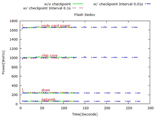
Figure 3: NPB: CG power consumption on 1024, 2048, 4096 and 8192 nodes respectively. “w/o FTI” denotes
experiment without checkpoints and faults. “w/ FTI(1,2,3,4)” denotes experiment with FTI and the checkpoint-
ing frequencies from level 1 to level 4 are 1, 2, 3 and 4 respectively. “w/ FTI(1,2,3,4) I” denotes the experiment
with FTI and inject faults.

                                               3. ANALYSIS
3.1 NPB benchmarks
For NPB benchmarks, we choose the largest problem size E to do all the experiments.
    In order to show the fault tolerance influence on power consumption, each application ran three times with the
same settings, except the checkpoints and faults. The first run records the power information without checkpoints
and faults. The second run adds checkpoints but no injected faults. The third run adds both checkpoints and
injected faults.
    Figure 1 and figure 2 presents the effects of checkpoints on execution time and energy consumption respec-
tively.
   The following subsection gives more detailed analysis on these three benchmarks.

3.1.1 CG
Figure 3 and figure 4 show the CG program power consumption on 1024, 2048, 4096 and 8192 nodes respectively.
CG programs ran at four scales. They are 1k, 2k, 4k and 8k nodes, which means 1k, 2k, 4k and 8k MPI ranks
separately. Since chip core, dram, networks consume most energy and checkpoints and faults do not significant
influences on other domains, we ignore other domains.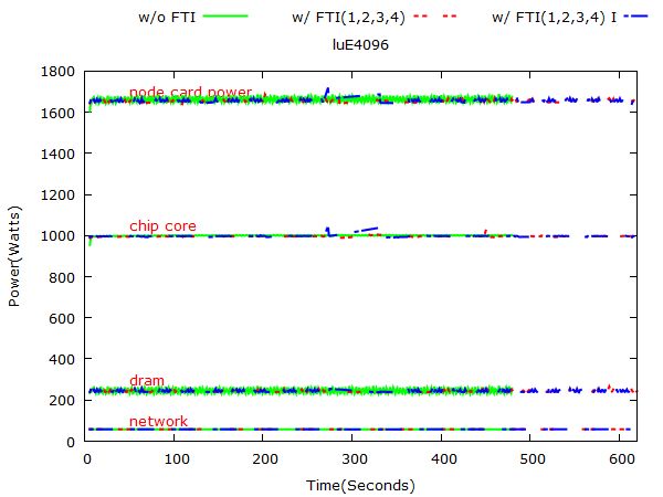
Figure 4: Box plot comparison of average power consumption at the node card level for NPB: CG.

             Figure 5: NPB: FT power consumption on 1024, 2048 and 4096 nodes respectively.

3.1.2 FT
Figure 5 and 6 show FT’s power consumption on different problem sizes. The FT experiment ran on 1k, 2k,
and 4k nodes. We skip the experiment on 8k nodes, because FT experiment on 8k nodes is too short to gather
enough power consumption information.

      Figure 6: Box plot comparison of average power consumption at the node card level for NPB: FT.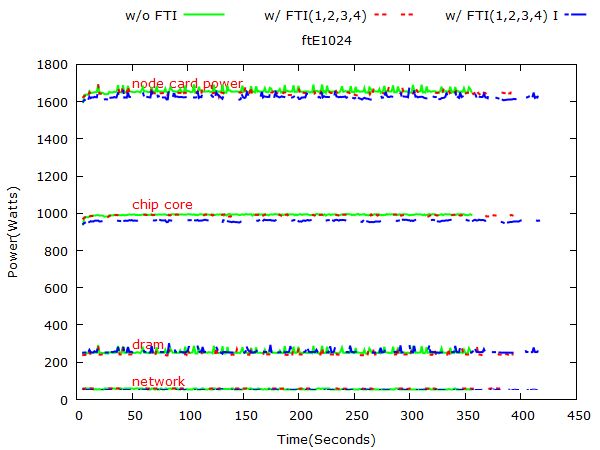
Figure 7: NPB: LU power consumption on 1024, 2048, 4096 and 8192 nodes respectively.

3.1.3 LU
Figure 7 and 8 show LU’s power consumption on different problem sizes.

3.2 Flash
In-build checkpoint option in flash code enables us doing checkpoint at regular time or instruction intervals. In
this experiment, we compare the power consumption of Sedov ran on 512 nodes with checkpoints and that with
checkpoints.
   Figure 9 presents the execution time and energy consumption of Flash: Sedov application.
   Figure 10 represents Flash’s power consumption at 512 scale.

3.3 STREAM
Note that for STREAM, FTI is used to do regular checkpoints and random fault injection. Figure 11 presents
the execution time and energy consumption of STREAM.
   Figure 12 represents STREAM’s power consumption on 32 nodes.

3.4 Key Observations
Based on the comprehensive analysis on NPB, Flash, and Stream benchmarks, we summarize the key observations
with the follwing five categories.
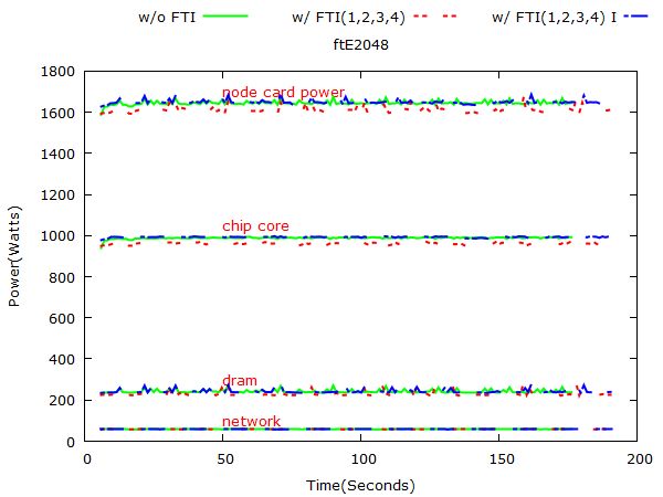
Figure 8: Box plot comparison of average power consumption at the node card level for NPB: LU.

             Figure 9: The execution time and energy of Flash: Sedov application.

                   Figure 10: Flash: Sedov power consumption at 512 scale.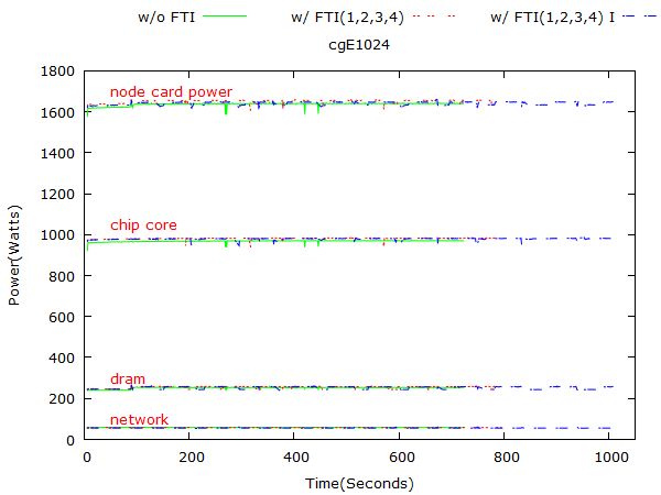
Figure 11: The execution time and energy of STREAM benchmark.

                            Figure 12: STREAM power consumption on 32 nodes.

3.4.1 With checkpoint or without checkpoint
   • The power consumption remains the same or reduces a little(-3.58% -0.24%) in most cases by adding
     checkpoint without injecting faults. The possible reason is that checkpointing is not computation intensive
     task, hence the chip core power is reduced in most cases, which causes the total power reduced too. There
     are only four exceptions, which are luE1024, luE2048, ftE2048 and cgE1024, but the differences are trivial
     and have not exceeded 1% in all three cases.
   • The execution time and energy increase after adding checkpoints. Adding the checkpoints with the same
     frequencies have the different effect on different application and even the same application running on
     different scales. For NPB benchmarks, the increases in the time range from 6.41% to 38.85% and the
     increases in the energy range from 4.17% to 27.95%. We can see from figure 7, that the energy cost is
     close related to execution time and they follow the same trend. For Stream benchmark, the execution
     time increase 33.15% and the energy increases 31.99% by adding checkpoints. Stream benchmark is more
     sensitive to the checkpoints. This is because Stream is a memory-intensive application. There is no local
     disk on nodes, FTI saves the level 1, 2 and 3 checkpoints in memory, which cause the competition between
     the checkpoint and progress of stream and we can observe the higher DRAM power than other benchmarks
     in this study. Hence, we observe more significant influence on Stream benchmark comparing with NPB
     benchmarks.

3.4.2 Inject fault or not
   • Injecting faults cause the power increases or remain the same(-0.68% 3.76%) in most cases comparing
     to only adding checkpoints without faults. The main increases came from the chip core power increases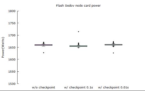
because the recovery process is computationally intensive. From Table 1, we observe that CG and LU
     average power on all 4 different scales increase the power consumption. Adding faults seems to reduce the
     power consumption for FT, this is because FT benchmark runs too short, that these two experiments do a
     different number of the four-level checkpoint and the difference of the number of checkpoints have a great
     influence on the short jobs. Stream benchmark and Flash benchmark also show the same trend.

   • Another finding is that injecting faults make the power consumption fluctuate. We can see it from the
     boxplots. It is clear that there are more outliers for power consumption with fault injections. There
     are more spikes after injecting faults. The recovery process first retrieves information from disk then re-
     computes from the latest checkpoint. The retrieving process is the not computationally intensive, but the
     re-computation is. The interruption of faults explains why there are more ups and downs when injecting
     faults.

   • Randomly injected faults have different effects on execution time and energy. Figure 7 shows that injected
     faults make the execution time of cgE1024, ftE4096 and luE8192 increase significantly. The logs of these
     runs show that all these runs experienced the fault error and recovered from level 4 checkpoint, which is
     the most time-consuming recovery process. Another observation is that as the number of nodes increases,
     the recovery process takes more time. For example, a fault error of luE8192 takes 90.69% more than that
     without error.
   • If we ignore the cases that experienced a fatal error, FTI is very efficient in recovery. The incremental
     percentage of execution time is ranging from 0.30% to 6.27% and that of energy is ranging from 0.31%
     to 4.79%. In reality, the failure rate is lower than the rate in our experiment, because we injected faults.
     Hence, we can say that if there are no errors that requiring all the nodes back to last checkpoints, faults
     have a trivial effect on execution time and energy. Stream also shows the same feature that injects faults
     without a fatal error does not affect the execution time and energy too much.

3.4.3 Number of nodes
   • For CG and FT, increasing the number of nodes seems further lowered the power with checkpointing
     comparing to that without checkpointing. The difference may be the result of the communication delay
     by introducing checkpoint. Level 2 and level 3 require storing checkpoints at other nodes, which involves
     the network. More nodes mean there are more communication and information needed to transfer in the
     system, which may delay the computation. As the result, the chip core power goes down as the number of
     node increases.

3.4.4 Energy
   • From the energy figures and Table 1, we can see that running application without checkpoints consumes
     less energy than running the same application with checkpoints. It is also true that application with fault
     injection consumes more energy than application without fault injection.

3.4.5 Time
   • The column plots present that running application without checkpoint takes less time and running appli-
     cation with fault takes more time than that without faults.
   • The time has a dominate role in energy. Although larger scale results in shorter execution time, the total
     energy consumed by application increase as the scale becomes larger. From energy usage view, smaller
     scale help saves energy.

                                            4. CONCLUSION
In this paper, we have analyze the effect of application checkpoints on power consumption. The observations
provides insight to design power- and checkpoint-aware scheduling policies.
REFERENCES
[1] Wallace, S., Z. Zhou, V. V., Coghlan, S., Tramm, J., Lan, Z., and Papka, M. E., “Application power profiling
on ibm blue gene/q,” in [IEEE International Conference on Cluster Computing (CLUSTER) ], (2013).
[2] “NAS Parallel Benchmarks.” https://www.nas.nasa.gov/software/npb.html. (Accessed: 27 August
2021).
[3] “Flash.” http://flash.uchicago.edu/site/. (Accessed: 27 August 2021).
[4] “Stream.” https://www.cs.virginia.edu/stream/. (Accessed: 27 August 2021).
[5] “Fault Tolerance Interface (FTI).” http://leobago.com/projects/. (Accessed: 27 August 2021).
[6] Di, S., Bautista-Gomez, L., and Cappello, F., “Optimization of multi-level checkpoint model with uncer-
tain execution scales,” in [Proceedings of the International Conference for High Performance Computing,
Networking, Storage and Analysis (SC) ], (2014).
[7] Fan, Y., Rich, P., Allcock, W., Papka, M., and Lan, Z., “Trade-Off Between Prediction Accuracy and
Underestimation Rate in Job Runtime Estimates,” in [CLUSTER ], (2017).
[8] Qiao, P., Wang, X., Yang, X., Fan, Y., and Lan, Z., “Preliminary Interference Study About Job Placement
and Routing Algorithms in the Fat-Tree Topology for HPC Applications,” in [CLUSTER ], (2017).
[9] Allcock, W., Rich, P., Fan, Y., and Lan, Z., “Experience and Practice of Batch Scheduling on Leadership
Supercomputers at Argonne,” in [JSSPP ], (2017).
[10] Li, B., Chunduri, S., Harms, K., Fan, Y., and Lan, Z., “The Effect of System Utilization on Application
Performance Variability,” in [ROSS], (2019).
[11] Fan, Y., Lan, Z., Rich, P., Allcock, W., Papka, M., Austin, B., and Paul, D., “Scheduling Beyond CPUs for
HPC,” in [HPDC ], (2019).
[12] Yu, L., Zhou, Z., Fan, Y., Papka, M., and Lan, Z., “System-wide Trade-off Modeling of Performance, Power,
and Resilience on Petascale Systems,” in [The Journal of Supercomputing], (2018).
[13] Fan, Y. and Lan, Z., “Exploiting Multi-Resource Scheduling for HPC,” in [SC Poster], (2019).
[14] Qiao, P., Wang, X., Yang, X., Fan, Y., and Lan, Z., “Joint Effects of Application Communication Pattern,
Job Placement and Network Routing on Fat-Tree Systems,” in [ICPP Workshops], (2018).
[15] Fan, Y., Lan, Z., Childers, T., Rich, P., Allcock, W., and Papka, M., “Deep Reinforcement Agent for
Scheduling in HPC,” in [IPDPS ], (2021).
[16] Fan, Y. and Lan, Z., “DRAS-CQSim: A Reinforcement Learning based Framework for HPC Cluster Schedul-
ing,” in [Software Impacts], (2021).
[17] Fan, Y., Rich, P., Allcock, W., Papka, M., and Lan, Z., “ROME: A Multi-Resource Job Scheduling Frame-
work for Exascale HPC System,” in [IPDPS poster], (2018).You can also read