Application of the Complete Data Fusion algorithm to the ozone profiles measured by geostationary and low-Earth-orbit satellites: a feasibility ...
←
→
Page content transcription
If your browser does not render page correctly, please read the page content below
Atmos. Meas. Tech., 14, 2041–2053, 2021
https://doi.org/10.5194/amt-14-2041-2021
© Author(s) 2021. This work is distributed under
the Creative Commons Attribution 4.0 License.

Application of the Complete Data Fusion algorithm to the ozone
profiles measured by geostationary and low-Earth-orbit
satellites: a feasibility study
Nicola Zoppetti1 , Simone Ceccherini1 , Bruno Carli1 , Samuele Del Bianco1 , Marco Gai1 , Cecilia Tirelli1 ,
Flavio Barbara1 , Rossana Dragani2 , Antti Arola3 , Jukka Kujanpää4 , Jacob C. A. van Peet5,6 , Ronald van der A5 , and
Ugo Cortesi1
1 Istituto
         di Fisica Applicata “Nello Carrara” del Consiglio Nazionale delle Ricerche, Via Madonna del Piano 10,
50019 Sesto Fiorentino, Italy
2 European Centre for Medium-Range Weather Forecasts, Shinfield Park, Reading, RG2 9AX, UK
3 Finnish Meteorological Institute, Atmospheric Research Centre of Eastern Finland, P.O. Box 1627, 70211 Kuopio, Finland
4 Finnish Meteorological Institute, Space and Earth Observation Centre, P.O. Box 503, 00101 Helsinki, Finland
5 Royal Netherlands Meteorological Institute, Utrechtseweg 297, 3731 GA De Bilt, the Netherlands
6 Vrije Universiteit Amsterdam, Department of Earth Sciences, 1081 HV, Amsterdam, the Netherlands

Correspondence: Nicola Zoppetti (n.zoppetti@ifac.cnr.it) and Simone Ceccherini (s.ceccherini@ifac.cnr.it)

Received: 15 November 2019 – Discussion started: 18 December 2019
Revised: 10 November 2020 – Accepted: 11 November 2020 – Published: 12 March 2021

Abstract. The new platforms for Earth observation from            profile measurements simulated in the thermal infrared and
space are characterized by measurements made at great spa-        ultraviolet bands in a realistic scenario. Following this, the
tial and temporal resolutions. While this abundance of infor-     fused products are compared with the input profiles; com-
mation makes it possible to detect and study localized phe-       parisons show that the output products of data fusion have
nomena, it may be difficult to manage this large amount of        smaller total errors and higher information contents in gen-
data for the study of global and large-scale phenomena.           eral. The comparisons of the fused products with the fusing
   A particularly significant example is the use by assimila-     products are presented both at single fusion grid box scale
tion systems of Level 2 products that represent gas profiles in   and with a statistical analysis of the results obtained on large
the atmosphere. The models on which assimilation systems          sets of fusion grid boxes of the same size. We also evaluate
are based are discretized on spatial grids with horizontal di-    the grid box size impact, showing that the Complete Data Fu-
mensions of the order of tens of kilometres in which tens or      sion method can be used with different grid box sizes even if
hundreds of measurements may fall in the future.                  this possibility is connected to the natural variability of the
   A simple procedure to overcome this problem is to extract      considered atmospheric molecule.
a subset of the original measurements, but this involves a loss
of information. Another option is the use of simple averages
of the profiles, but this approach also has some limitations
that we will discuss in the paper. A more advanced solution is    1   Introduction
to resort to the so-called fusion algorithms, capable of com-
pressing the size of the dataset while limiting the information   In the context of the Copernicus programme (https://www.
loss. A novel data fusion method, the Complete Data Fusion        copernicus.eu, last access: 29 December 2020) coordinated
algorithm, was recently developed to merge a set of retrieved     by the European Commission, the European Space Agency is
products in a single product a posteriori. In the present pa-     responsible for the Space Component, consisting of a novel
per, we apply the Complete Data Fusion method to ozone            set of Earth Observation (EO) satellite missions for environ-
                                                                  mental monitoring applications: the Sentinel missions (https:

Published by Copernicus Publications on behalf of the European Geosciences Union.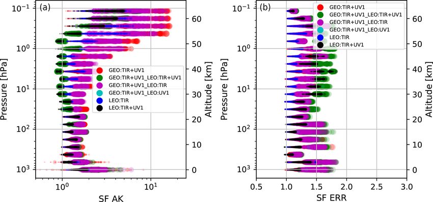
2042                                   N. Zoppetti et al.: Application of the CDF algorithm to GEO and LEO ozone profiles

//sentinel.esa.int/web/sentinel/missions, last access: 29 De-        rithms to ozone profiles simulated according to specifications
cember 2020). Each mission focuses on a specific aspect of           similar to those of the atmospheric Sentinels.
EO. In particular, the geostationary (GEO) mission Sentinel-            The use of synthetic data allows for evaluating the per-
4 and the two low-Earth-orbit (LEO) missions (Sentinel-5p            formances of the algorithms in terms of differences between
and Sentinel-5), referred to as the atmospheric Sentinels, are       the products and a reference truth, represented by the atmo-
dedicated to monitoring air quality, stratospheric ozone, ul-        spheric scenario used in the L2 simulation procedure. On the
traviolet surface radiation and climate.                             other hand, the absence of systematic errors in the simulated
   The atmospheric Sentinels will provide an enormous                measurements limits the study to ideal measurement condi-
amount of data with unprecedented accuracy and spatio-               tions. However, the CDF algorithm intrinsically provides a
temporal resolution. In this scenario, a central challenge is        mechanism to include different kinds of errors in the analy-
to enable a generic data user (for example, an assimilation          sis. For instance, Ceccherini et al. (2018) discussed how to
system) to exploit such a large amount of data.                      treat interpolation and coincidence errors, while Ceccherini
   A variety of approaches can serve the purpose of convey-          et al. (2019) explicitly introduce the treatment of systematic
ing, in a single product, the information associated with re-        errors.
mote sensing observations of the vertical distribution of a             This work is divided into two parts. In the first part, we
given atmospheric target from multiple independent sources.          describe the datasets and methodologies (the L2 simulation
Strategies for the combined use of multiple atmospheric pro-         procedure and the CDF) and discuss the differences between
file datasets include a posteriori data fusion techniques, syn-      CDF and mere averaging. In the second part, the quality of
ergistic inversion processes (Aires et al., 2012 and references      the fused products obtained from L2 profiles that are not per-
therein; Natraj et al., 2011; Cuesta et al., 2013; Cortesi et al.,   fectly co-located in space and in time is analysed. To account
2016; Sato et al., 2018) and, in broader terms, might include        for the geo-temporal differences in the L2 profiles, a coinci-
assimilation systems (Lahoz and Schneider, 2014).                    dence error is added to the fused product error budget. The
   The three approaches differ in the accepted inputs and in         fused and standard L2 products are compared and assessed
the involved models. In the synergistic inversion, the inputs        in terms of their information content, highlighting the better
consist of the radiance observations (Level 1 products) of all       data quality provided by the fusion. Finally, we also show
the measurements, and the output profiles are obtained by a          that the CDF can be applied with different coincidence grid
simultaneous retrieval of these observations. A posteriori fu-       box sizes, allowing for different compression factors of the
sion techniques consist of sophisticated averaging processes         Level 2 input data volume.
in which the inputs are profiles (Level 2 products) retrieved           Some of the characteristics of the products used in this
from the single measurements. The assimilation techniques,           work differ from what they will be in reality: in particular, the
in their more general implementations, can accept both radi-         spatial sampling (spacing between pixels and shape) and in
ances and profiles as inputs and use the information of the          some cases the signal-to-noise ratio (GEO-TIR instrument)
measurements as inputs of an atmospheric model. Each of              of the instruments used in the present paper (both GEO and
these strategies implies different advantages and drawbacks,         LEO) are different from those of that will be onboard the
ultimately assessing the cost-to-benefit ratio that drives the       Sentinel 4/MTG-S and EPS-SG. Nevertheless, this work fo-
selection of the option of choice for the specific case under        cuses on a comparison of the fused and L2 products and,
investigation.                                                       in particular, on the ability of the CDF to induce quality im-
   In particular, data fusion algorithms, such as the Complete       provements that are, in some sense, independent from precise
Data Fusion (CDF) algorithm (Ceccherini et al., 2015), can           instrumental characteristics.
be well suited to reducing the data volume that users need to           The application of CDF to L2 products simulated with the
access and handle while retaining the information content of         characteristics that are even only similar to the ones expected
the whole Level 2 (L2) product.                                      from the atmospheric Sentinel 4 and 5 products allows for
   The CDF inputs are any number of L2 profiles retrieved            establishing the possible benefits in the case of real Sentinel
with the optimal estimation technique and characterized by           data.
their a priori information, covariance matrix (CM) and aver-
aging kernel (AK) matrix. The output of the CDF is a single
product (also characterized by a priori, CM and AK matri-            2     Material and methods
ces) in which the vertical sensitivity increases and the error
reduces with respect to the inputs (Ceccherini et al., 2015).        2.1    Atmospheric scenario and ozone climatology
   This work is based on the simulated data produced in the
context of the Advanced Ultraviolet Radiation and Ozone              In this work, we used two basic external sources to generate
Retrieval for Applications project (AURORA; Cortesi et al.,          the database of the standard L2 ozone products: the ozone
2018), funded by the European Commission in the frame-               climatology and the atmospheric scenario.
work of the Horizon 2020 programme. The project regards                 We used the ozone climatology as a priori information in
the sequential application of fusion and assimilation algo-          both the simulation of L2 products and the CDF. The atmo-

Atmos. Meas. Tech., 14, 2041–2053, 2021                                               https://doi.org/10.5194/amt-14-2041-2021
N. Zoppetti et al.: Application of the CDF algorithm to GEO and LEO ozone profiles                                               2043

spheric scenario represents the true state of the atmosphere,        taken from a Gaussian distribution with average equal to zero
and we used it in both the simulation of L2 products and the         and CM given by Sy :
quality assessment of the fused ones.                                                      −1
   In particular, the ozone climatology was derived from             δ = Gε = KT S−1     −1
                                                                                                KT S−1
                                                                                  y K + Sa          y ε.                           (3)
McPeters and Labow (McPeters and Labow, 2012) and di-
rectly provided the a priori profile x a used either in the simu-    The CM S associated with the retrieval error δ (introduced in
lation equations (Eq. 1) or in the fusion equation (see Eq. 6).      Eq. 3) is given by Eq. (4) (Rodgers, 2000):
We calculate the diagonal terms of the a priori CM Sa as
the square of the SD of McPeters and Labow climatology,              S = hδδ T i
putting an inferior limit to this diagonal value equal to the                             −1                     −1
square of 20 % of the a priori profile. The off-diagonal ele-          = KT S−1         −1
                                                                                 y K + Sa      KT S−1   T −1     −1
                                                                                                   y K K Sy K + Sa      .          (4)
ments are calculated using a correlation length of 6 km. The
correlation length is used to reduce oscillations in the sim-           The CM Stotal associated with the total error δ total (i.e. the
ulated profiles, and 6 km is the typical value used for nadir        difference between the simulated and the true profiles, equal
ozone profile retrieval (Liu et al., 2010; Miles et al., 2015).      to the random δ plus the so-called smoothing error, caused by
The a priori CM is used in the equation of the L2 AK ma-             the limited vertical resolution of the measurement; see Eq. 7),
trix (Eq. 2) and in Eqs. (4) and (5) of the next paragraph.          is given by Eq. (5) (Rodgers, 2000):
The a priori CM Sa also plays an important role in the CDF                                                       −1
equations (see Eq. 6).                                               Stotal = hδ total δ Ttotal i = KT S−1     −1
                                                                                                        y K + Sa      .            (5)
   The atmospheric scenario is taken from the Modern Era-
Retrospective analysis for Research and Applications ver-               It should be noted that through the term δ it is possible to
sion 2 (MERRA-2) reanalysis (Gelaro et al., 2017). The               simulate additional error components with respect to the ran-
MERRA-2 data are provided by the Global Modelling and                dom one considered in this study, and this fact adds flexibility
Assimilation Office (GMAO) at NASA Goddard Space                     to the simulation method.
Flight Center. This reanalysis covers the recent time of re-            In this study, we use the above formulation to simulate
motely sensed data, from 1979 through the present. The at-           ozone profiles in two spectral bands (UV1 and TIR) for both
mospheric scenario is the source of true profile xt used in          GEO and LEO, after considering the instrument specifica-
Eq. (1) to synthesize the simulated L2 products and repre-           tions and accounting for the differences in the two spectral
sents the main reference for the comparison of the quality of        bands. In particular, considering a fixed geolocation, true
L2 and fused products.                                               profile and a priori information, we obtain the L2 products
                                                                     of the different instruments by choice of K and Sy , that have
2.2   L2 product simulation algorithm
                                                                     been synthesized using the technical requirements of the con-
                                                                     sidered platforms and their foreseen performances.
The simulation algorithm was originally formalized in the
context of the AURORA project, aiming at an efficient com-           2.3   L2 product technical specifications
putational process. The L2 retrieved state is simulated on a
fixed vertical grid with a 3 km step by the linear approxima-        In the context of Sentinel missions, the ozone profiles derived
tion given in Eq. (1):                                               from measurements in the UV region will be retrieved from
                                                                     spectral radiances acquired by the UVNS/Sentinel-5 spec-
x̂ = Ax t + (I − A)x a + δ.                                   (1)    trometer onboard the Meteorological Operational satellite–
                                                                     Second Generation (MetOp-SG) and by the UVN/Sentinel-
   In Eq. (1), x t is the true state of the atmosphere represented
                                                                     4 spectrometer onboard the Meteosat Third-Generation
by the atmospheric scenarios, x a is the a priori estimate of
                                                                     Sounder (MTG-S). For ozone and other targets observed in
the state vector provided by the ozone climatology, δ is the
                                                                     the TIR, the atmospheric Sentinel missions will use the op-
uncertainty in the retrieved value due to measurement noise
                                                                     erational products of IASI-NG on MetOp-SG and IRS on
and A = ∂ x̂/∂x t is the AK matrix (Rodgers, 2000) calculated
                                                                     MTG.
according to Eq. (2).
                                                                        In the framework of the AURORA project, we simulated
                  −1                                               ozone products from the instruments mentioned above by us-
A = KT S−1
        y  K + S−1
                a      KT S−1
                           y K                                (2)    ing the information available at the beginning of 2016 (ESA,
                                                                     2011, 2012; EUMETSAT, 2010; Crevoisier et al., 2014). We
In Eq. (2), K is the Jacobian matrix of the forward model,           applied some simplifications to these specifications: for ex-
the superscript T is the transpose operator, Sy is the CM of         ample, we considered only the UV1 band (neglecting UV2,
the observations and Sa is the CM of the a priori profile. The       300–320 nm), simplified spatial sampling (spacing between
retrieval error δ is calculated by applying the gain matrix G        pixels and shape) and in some cases a different signal-to-
(Rodgers, 2000) to an error ε on the observations randomly           noise ratio (GEO-TIR L2 type, see Table 1). Consequently,

https://doi.org/10.5194/amt-14-2041-2021                                                Atmos. Meas. Tech., 14, 2041–2053, 2021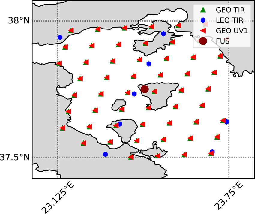
2044                                             N. Zoppetti et al.: Application of the CDF algorithm to GEO and LEO ozone profiles

the dataset of simulated L2 products is not exactly in line                        Concerning the profile and the error, we can consider the
with the specifications currently foreseen for the instruments                  CDF as a “smart average” in which the a priori information
of interest. Table 1 reports some of the more relevant char-                    is removed from the L2 profiles and CMs before they are
acteristics of the simulated measurements. It is worth noting                   put together in the average. The total error of the L2 product
that when an instrumental parameter has both a goal value                       without a priori is higher than the original one, and the effect
(the value in case the instrument performs at its best) and a                   of the average only partially compensates this error increase.
threshold value (the value that we expect to reach anyhow),                     Consequently, even if the total error of the fused product is
the latter is used for the simulation.                                          generally lower than the one of the single L2 fusing prod-
   A more detailed description of the instrumental and ob-                      uct, it is in general higher than the error of the average. The
servational features goes beyond the scope of this article.                     behaviour of the AK matrix is less intuitive, and we will thor-
All the relevant information was reported in the Technical                      oughly analyse it in the presentation of the results.
Note on L2 data simulations (AURORA, 2017) and can also                            If the input products are not coincident in time and space,
be found in Cortesi et al. (2018). In the following sections                    the CDF introduces a coincidence error characterized by a
of this paper, we do not directly refer to the reference in-                    CM Scoinc . In this work, we calculated the diagonal elements
struments names, but we use an alternative nomenclature:                        of Scoinc as the square of 5 % of the a priori profile x a , where
specifically, we refer to UVNS/MetOp-SG as LEO-UV1, to                          we choose this value considering the size of the coincidence
UVN/MTG as GEO-UV1, to IASI-NG/MetOp-SG as LEO-                                 grid cells used in this study. We calculate the off-diagonal
TIR and IR/MTG as GEO-TIR. Since we simulated instru-                           elements of Scoinc , applying an exponential decay with a cor-
ments with characteristics that differ from the real specifica-                 relation length of 6 km (Ceccherini et al., 2018). The 5 %
tions, we think it is appropriate to also use an independent                    choice matured in a heuristic way by varying the percentage
terminology to avoid misunderstandings.                                         value, observing the quality of the fused product in single
                                                                                reference cells, and by looking at the entire dataset in repre-
2.4    The CDF method                                                           sentations similar to Figs. 6 and 7.
                                                                                   The dynamical choice of Scoinc is presented in Ceccherini
In this section, we briefly recall the formulas of the CDF                      et al. (2019). Specifically, the a priori error (coincident with
method (Ceccherini et al., 2015). We assume N indepen-                          the climatological variability) is used as the reference for the
dent simultaneous measurements of the vertical profile of                       diagonal elements and a fixed exponential decay is applied
an atmospheric species that refer to the same geolocation.                      as well. However, the multiplicative factor is calculated by
Performing the retrieval of the N measurements, we obtain                       imposing the requirement the cost function of the retrieval
N vectors x̂ i (i = 1, 2, . . ., N ) that provide independent es-               be equal to its expected value. That study, which is based on
timates of the profile, here assumed to be represented on a                     simulated products similar to the ones of this work, shows
common vertical grid. Using these N measurements as in-                         that even if the coincidence error is strictly needed for the
puts, the CDF produces a single product characterized by a                      correct behaviour of the CDF product, this is not strongly de-
profile xf , an AK matrix Af and a CM matrix Sf as out-                         pendent on its exact amount until it is smaller than the errors
put, with the procedure summarized by Eq. (6). These three                      of the individual L2 products.
quantities are dependent on the input products, Ai and Si ,                        The formulae of Eq. (6) refer to cases of measurements
hereafter referred to as fusing products, and depend on the                     made on the same vertical grid. In general, an interpolation
a priori information (x a , Sa ) used as a constraint for the fused             error may also be needed, considering that the retrievals of
product.                                                                        the products to be fused can be defined on different verti-
                                                                                cal grids. In Ceccherini et al. (2018) the general equations of
                                                                                CDF in the case of the fusion of products characterized by
α i = x̂ i − (I − Ai )x ai = Ai x t + δ i + Ai δ coinc,i                 (6a)
                                                                                different vertical grids are presented and discussed together
S̃i = Si + Ai Scoinc,i ATi                                               (6b)   with the equation of the interpolation error that depends on
       XN                               −1                                    the involved grids and the AK matrices of the fusing prod-
xf =          i=1
                    ATi S̃−1      −1
                          i Ai + Sa                                             ucts. However, since the interpolation error does not apply to
           XN
                       T −1                    −1
                                                                               the present study (we simulated all the L2 products on the
         ·     i=1
                   A   i S̃   i    α   i +  S  a  x a                    (6c)   same vertical grid), it has not been considered in Eq. (6) or
        XN
                    T −1
                                                 −1 XN                         in the following discussion.
Af =         i=1
                 A  i  S̃ i      A   i  +  S −1
                                             a              AT S̃−1 Ai
                                                         i=1 i i
                                                                         (6d)
       XN
                   T −1
                                                 −1 XN                         2.5   Arithmetical average and biases
Sf =         i=1
                 A i  S̃ i      A   i  +  S −1
                                            a               AT S̃−1 Ai
                                                         i=1 i i
          XN                                     −1                           Before proceeding, it is necessary to clarify why the arith-
                     T −1                     −1
       ·      i=1
                  A  i  S̃ i      A   i  +  S a                          (6e)   metic average of the profiles cannot be considered as a good
            XN                                      −1                        option to represent a set of products retrieved with optimal
                            T −1                  −1
Sf total =       i=1
                       A    i   S̃i     A i +   S a                      (6f)   estimation techniques.

Atmos. Meas. Tech., 14, 2041–2053, 2021                                                           https://doi.org/10.5194/amt-14-2041-2021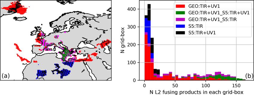
N. Zoppetti et al.: Application of the CDF algorithm to GEO and LEO ozone profiles                                                                                                               2045

Table 1. Instrument characterization relevant for the simulation process. Goal (G) and threshold (T ) values correspond, respectively, to
estimates of the parameters in the case that the instrument performs at its best and to limit values that we expect to reach anyhow. AURORA
will be using threshold values for the generation of simulated data.

    L2 type name                         GEO-TIR                        GEO-UV1                                         LEO-TIR                                   LEO-UV1
    Platform∗                                  Meteosat Third-Generation Sounder (MTG-S)                                       Meteorological Operational satellite–Second
                                                                                                                                        Generation (MetOp-SG)
    Reference instrument∗                Infrared Sounder               UV–VIS–NIR Sentinel-4                           Infrared Atmospheric                      UV–VIS–NIR–SWIR
                                         (IRS)                          spectrometer (UVN)                              Sounding Interferometer –                 Sentinel-5 spectrometer
                                                                                                                        New Generation (IASI-NG)                  (UVNS)

    Retrieval spectral range             1030–1080 cm−1                 305–320 nm                                      1030–1080 cm−1                            270–300 nm
    Spectral resolution                  0.625 cm−1                     0.5 nm                                          0.25 cm−1                                 1.0 nm
                                         (apodized IRSF)                                                                (apodized IRSF)
    Spectral sampling ratio              1                              3                                               2                                         3
    Noise-equivalent                     IRS1b                                                                          IRS2b
    brightness temperature
    scenario (according to
    Crevoisier et al. 2014)
    Signal-to-noise                                                     160 and 305 nm (T ),                                                                      100 and 270 nm (T , G)
    ratio radiance                                                      320 and 310 nm (T ),
                                                                        630 and 315 nm (T ),
                                                                        900 and 320 nm (T , G)
    Field of view                        15 km × 15 km (T ),            ≤ 8 km                                          12 km × 12 km (T ),                       50 km × 50 km (T ),
                                         5 km × 5 km (G)                at 45◦ N and 0◦ E (the longitude                5 km × 5 km (G)                           15 km × 15 km (G)
                                                                        of the satellite)
    Pixel size used in                                                  8 km                                            12 km                                     45 km
    the simulation (assumed
    square and nadir)
  ∗ The table entries in these rows are not meant to suggest that the specifications listed in this table refer directly to these instruments. Instead, the listed instruments are examples of
  instruments that are actually planned with similar (but slightly different) specifications.

   To do this, we consider N coincident L2 measurements                                                the information of several products into one. Further reasons
(i = 1, . . ., N ) referring to the same true profile, the same                                        concern the choice of a suitable AK matrix to be assigned
AK matrix and the same CM but having different (noise) er-                                             to the average (see also von Clarmann and Glatthor, 2019)
rors δ i randomly generated according to Eq. (3). The total                                            and the management of possible coincidence and interpola-
error equation for the ith measurement is given in Eq. (7)                                             tion errors. An explicative comparison of the application of
and can be easily derived from Eq. (1).                                                                CDF and standard averages in the case of 1000 coincident L2
                                                                                                       products is reported in the Supplement.
δ i,total = x̂ i − x t = (I − Ai )(x a − x t ) + δ i                                      (7)
    Considering that the individual measurements are co-
located in space and time, they thus refer to the same truth,                                          3     Results and discussion
the same a priori profile and the same AK matrix A; the mean
total error is equal to                                                                                3.1      Fusion in realistic spatial and temporal resolution
                                                                                                                conditions: the L2 datasets
                                                     1 XN
hδ i,total i = hx̂ i i − x t = (I − A)(x a − x t ) +       δ . (8)
                                                        i=1 i
                                                     N                                                 To analyse the behaviour of CDF in realistic spatial and tem-
    It follows that the averaging process reduces the random                                           poral resolution conditions, we consider four sets of mea-
component of the total error but does not reduce the bias                                              surements. These measurements correspond to the cloud-
due to the a priori information. This bias is equal to the term                                        free observations that were possible between 09:00 and
(I − A)(x a − x t ) of Eq. (8), which therefore becomes a dom-                                         10:00 UTC on 1 April 2012. Table 2 lists the L2 product
inant component as the number N increases. The existence                                               types, namely GEO-TIR, GEO-UV1, LEO-TIR and LEO-
of this bias is one of the reasons why the arithmetic aver-                                            UV1, used in this article. The L2 datasets have been gener-
age cannot be considered as a reference algorithm to collect                                           ated according to the Eqs. (1)–(5) described in Sect. 2.2. The

https://doi.org/10.5194/amt-14-2041-2021                                                                                           Atmos. Meas. Tech., 14, 2041–2053, 2021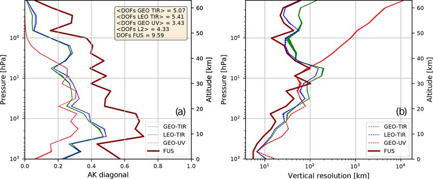
2046                                    N. Zoppetti et al.: Application of the CDF algorithm to GEO and LEO ozone profiles

Table 2. Number and horizontal resolution of the simulated mea-
surements. For the GEO platform across-track is a south–north di-
rection and along-track is an east–west direction.

      L2 type       Number of       Minimal distance between
                     simulated          measurements across
                  measurements           × along track (km)
      GEO-TIR             35 594
                                                      5.7 × 7.4
      GEO-UV1             35 594
      LEO-TIR              8023                    12.2 × 12.3
      LEO-UV1                570                   46.2 × 46.7
      TOTAL               79 781

details of the simulation process are explored in the Technical
Note (AURORA, 2017), considering that here we simulated
all the pixels corresponding to a clear sky line of sight in the
atmospheric scenario, without applying any additional selec-
                                                                       Figure 1. Geographical distribution of the simulated L2 measure-
tion criteria. In the AURORA project’s main work stream,
                                                                       ments and geolocation of the fused product. The dashed and dotted
we considered 4 months of data; however, we simulated only             black lines represent the borders of the 0.5◦ × 0.625◦ grid cells.
a subset of the clear-sky pixels to reduce the computational
cost of the simulations (Tirelli et al., 2020). In this AURORA
side study, we consider 1 h of data, and we simulate all the
clear-sky pixels without additional filters, choosing the orbits       ual profiles with their own, and presents a smaller estimated
so that GEO-LEO coincidences occur. Figure 5a indirectly               total error than the individual L2 products. In particular, the
represents the spatial distribution of the products simulated          Fig. 2b allows for seeing the performances of CDF in the
for this study.                                                        tropospheric region in detail.
                                                                          The retrieved profile representation is always a compro-
3.2    Single grid box analysis (0.5◦ × 0.625◦ )                       mise between the amplitude of the errors and the vertical
                                                                       resolution. The latter can be quantified by the AKs, which
We consider the case of a single grid box (Fig. 1). In the             ideally would be equal to the identity matrix in the case of
selected grid box, 118 measurements were available (55 of              a profile that has a vertical resolution equal to that defined
GEO-TIR, 55 of GEO-UV1, 8 of LEO-TIR and no LEO-                       by the sampling grid. Diagonal elements with values smaller
UV1). The cell is 0.5◦ in latitude and 0.625◦ in longitude,            than 1 correspond to a loss of vertical resolution. In Fig. 3b,
centred on Aegina in the Aegean Sea. The cell size has been            we compare the diagonal elements of the AKs of the L2
chosen to be comparable with the assimilation grid used in             products with the AK diagonal of the fused product. Here
the AURORA project. We assign the geolocation of the fused             we have also computed the number of degrees of freedom
product to be the barycentre of the horizontal coordinates of          (DOF), given by the sum of the diagonal elements of the AK
the L2 measurements in the grid box. In this particular case,          matrix (Rodgers, 2000), for both L2 and fused products and
since the horizontal distribution of the 118 L2 profiles is quite      reported the values in the text box in Fig. 3a. Note that the
homogeneous, the barycentre is placed at the centre of the             number of DOF of the fused product is about twice the num-
grid cell.                                                             ber of DOF of the best L2 product. In Fig. 3b, we compare
   Figure 2 shows with green lines the absolute (Fig. 2a) and          the vertical resolution profiles of L2 and fusion products. We
relative (Fig. 2b) differences between each L2 profile and             calculate the vertical resolution starting from AK matrices
the corresponding true profile, with a red line showing the            according to the full-width-at-half-maximum (FWHM) ap-
difference between the fused (FUS) profile and the mean                proach (Rodgers, 2000) and specifically with the algorithm
truth (computed as the average of the 118 true profiles), a            defined in Ridolfi and Sgheri (2009).
dashed and dotted black line showing the average of the es-               From the comparison of the Fig. 3a and b, it can be noted
timated SD of the total error of the individual L2 measure-            that the increase of the AK matrix diagonal values of FUS
ments σ total , and with a dashed and dotted red line showing          product, and consequently the increase of the number of
the estimated SD of the total error of the fused profile σ f total .   DOF, implies an improved vertical resolution only in a sub-
The last two quantities have been calculated as the square             set of the vertical levels. To better understand the effect of
root of the diagonals of the Stotal and Sf total CMs given by          the fusion on the AK matrices, it is useful to analyse the be-
Eqs. (5) and (6), respectively. Figure 2 shows that the fused          haviour of their rows. In Fig. 4, two rows are represented,
product is in better agreement with its truth than the individ-        one that refers to the troposphere (Fig. 4a, 6 km) and one the

Atmos. Meas. Tech., 14, 2041–2053, 2021                                                  https://doi.org/10.5194/amt-14-2041-2021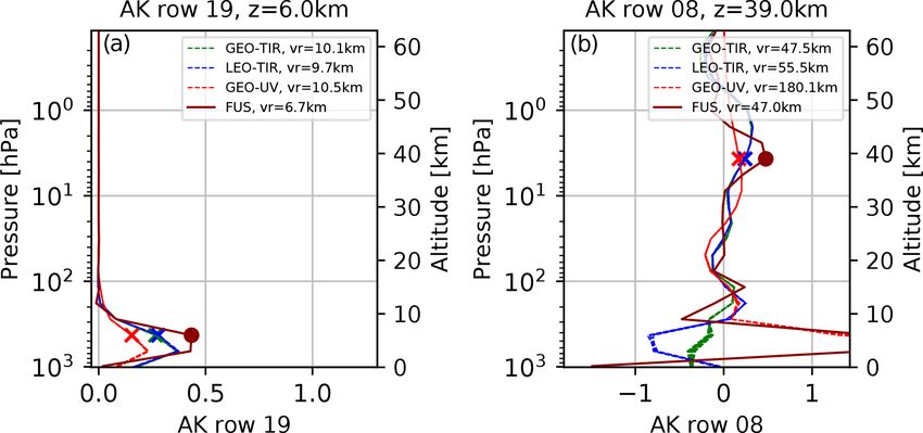
N. Zoppetti et al.: Application of the CDF algorithm to GEO and LEO ozone profiles                                                        2047

Figure 2. (a) The absolute differences between L2 profiles and their true profiles (green lines), the absolute difference between the fused
profile and the average of the true profiles (continuous dark red line), and the average of σ total of L2 simulations (dashed and dotted black
lines) and σ f total (dashed and dotted dark red lines). (b) The relative percentage differences between L2 profiles and their true profiles
(green lines), the relative percentage difference between the fused profile and the average of the true profiles (continuous dark red line), the
average of σ total of L2 simulations normalized with respect to the true profile and expressed in percentage (dashed and dotted black lines),
and σ f total normalized with respect to the true profile and expressed in percentage (dashed and dotted dark red lines).

Figure 3. (a) AK diagonals for the GEO-TIR products (red lines), LEO-TIR products (blue lines), GEO-UV products (red lines) and the
FUS product (dark red line). In the text box, the average number of DOF for each type of L2 product, the average number of DOF for all L2
products and the number of DOF of the FUS product are reported. (b) Vertical resolution (FWHM) profiles for the GEO-TIR products (red
lines), LEO-TIR products (blue lines), GEO-UV products (red lines) and the FUS product (dark red line). In each panel, while the solid dark
red line is a single one, the red and green lines are both 55 overlapped lines, and the blue lines are eight overlapped lines (one for each L2
product).

middle stratosphere (Fig. 4b, 39 km), where the reference al-             the vertical resolution with respect to L2 products. The sec-
titude is corresponding to the diagonal value of the row. The             ond phenomenon is linked to the fact that while for the FUS
value of the vertical resolution at the considered altitude is re-        product the maximum value of the AK row corresponds to
ported in the legend (the minimum vertical resolution at the              its diagonal element, for the L2 products these maxima are
considered vertical level for each type of L2 product), and               shifted with respect to the reference altitude of the rows. The
the diagonal value of each row is evidenced in the graphs                 last phenomenon is a stronger contribution of the (simulated)
with cross (L2) and dot markers (FUS). At lower altitudes                 measurements with respect to the a priori values in the FUS
(Fig. 4a), the DOF increase can be attributed to three distinct           product, where the latter effect can be evidenced by consid-
phenomena. The first is the constriction of the main FUS AK               ering the sum of all the elements of the rows that assume
lobe and the consequent improvement (of more than 30 %) of                0.913 as the maximum value for the L2 products and 0.956

https://doi.org/10.5194/amt-14-2041-2021                                                      Atmos. Meas. Tech., 14, 2041–2053, 2021
2048 N. Zoppetti et al.: Application of the CDF algorithm to GEO and LEO ozone profiles
Figure 4. (a) Rows of AK matrices at 6 km. (b) Rows of AK matrices at 39 km GEO-TIR products (red lines), LEO-TIR products (blue
lines), GEO-UV products (red lines) and the FUS product (dark red line).
for the FUS product. In this particular case, all these three are characterized by a small number of L2 measurements,
effects go in such a direction that they can be considered while when GEO products are present, many L2 measure-
benefits of CDF application. The results at higher altitudes ments can be present.
(39 km, Fig. 4b) are primarily influenced by the shape of the With the selected grid box size and the multitude of dif-
AK rows that exhibit large secondary lobes that degrade the ferent products that are present in each cell, the question is
vertical resolution. which product can be used in alternative to the fusion process
in those operations in which a single product is requested in
3.3 Statistical analysis for a large domain each grid box. Since the averaging process is affected by a
large bias error, a viable alternative is the use of the best
While the analysis of the previous paragraph focuses on a fusing product present in the cell, and we want to compare
particular grid box, here an analysis of the CDF behaviour is the CDF result with this product. This comparison is the so-
presented, referring to all the 1939 fusion grid boxes in which called Synergy Factor (SF), introduced by Aires et al. (2012).
more than one of the 79 781 L2 simulated products consid- Although Aires introduces SF only for errors (Eq. 11), we ex-
ered in Table 2 is placed. The fused products can be classified tend their definition to include other quantities because they
depending on the types of L2 measurements falling inside the constitute a useful tool to synthetically represent the perfor-
coincidence grid cell. Since GEO-TIR and GEO-UV1 prod- mances of fusion algorithms.
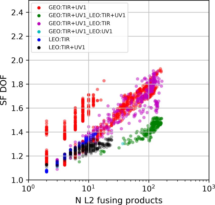
ucts are in perfect coincidence and LEO-UV1 products have The SF DOF, defined by Eq. (9), is the ratio between the
a horizontal spacing larger than the cell size, only six fused number of DOF of the FUS product, and the maximum num-
product types (FUS type), listed in Table 3, effectively occur. ber of DOF of L2 fusing products. In this equation, the in-
In this table, the FUS type and its description are reported dex l enumerates the vertical levels and the index i enumer-
together with the following complementary data: ates the L2 products fused in each grid box.
– N cells, i.e. the number of grid boxes characterized by P
the considered FUS type. l Af,ll
SF DOF = P (9)
max l All
i∈L2
– < NL2 >, i.e. the mean number of individual L2 fusing
profiles per grid box. When SF DOF is larger than 1.0, the FUS product carries
more information than the individual L2 measurements. Fig-
– Max NL2, i.e. the maximum number of individual L2
ure 6 shows that the SF DOF computed for all the fused prod-
fusing products per grid box.
ucts (and plotted as a function of the number of L2 profiles
Figure 5a shows the geographical distribution of the FUS in each grid box) is always larger than 1.0. It is also worth
products. Different colours have been used to classify the noticing that SF DOF increases approximately linearly with
fused data according to their provenance type. The irregular the logarithm of the number of fusing products, although
geographical coverage is due to the realistic distribution of the proportionality depends on the FUS type. The two dif-
the cloud-free measurements. The histogram in the Fig. 5b ferent clusters of red symbols (GEO:TIR + UV1) are caused
shows the number of cells that contain a given number of by the different latitude bands in which these products are
measurements, divided into different colours depending on distributed (see also Fig. 5a). It is important to underline that
the FUS type. The FUS cells in which only LEO products fall the improvement in vertical resolution is the most demanding
Atmos. Meas. Tech., 14, 2041–2053, 2021 https://doi.org/10.5194/amt-14-2041-2021N. Zoppetti et al.: Application of the CDF algorithm to GEO and LEO ozone profiles 2049
Table 3. Types and characteristics of the fused product when a coincidence grid cell size of 0.5◦ × 0.625◦ is used. Ncells is the number of grid
boxes characterized by the considered FUS type, < NL2 > is the mean number of individual L2 fusing profiles per grid box and maxNL2 is
the maximum number of individual L2 fusing products per grid box.
FUS type Description Ncells < NL2 > maxNL2
GEO:TIR + UV1 Two or more GEO pixels, no LEO pixels. 908 29.3 160
GEO:TIR + UV1_LEO:TIR + UV1 Two or more GEO pixels, one or more LEO-TIR pixel, 245 114.7 163
one or more LEO-UV1 pixel.
GEO:TIR + UV1_LEO:TIR Two or more GEO pixels, one or more LEO-TIR pixel, 299 69.4 165
no LEO-UV1 pixels.
GEO:TIR + UV1_LEO:UV1 Two or more GEO pixels, one or more LEO-UV1 pixel, 2 20 37
no LEO-TIR pixels.
LEO:TIR + UV1 No GEO pixels, one or more LEO-TIR pixels, 247 11.1 24
one or more LEO-UV1 pixels.
LEO:TIR No GEO pixels, two or more LEO-TIR pixels, 238 6.2 14
no LEO-UV1 pixels.
Total 1939 41.1 165
Figure 5. (a) Geographical distribution of FUS products differentiated by FUS type where the effect of the lower resolution of LEO-UV1
with respect to the other L2 products is the cause of the periodic FUS type transitions in the Mediterranean area. (b) Histogram of the number
of cells with a given number of L2 measurements differentiated by FUS type.
requirement in remote sensing observations and, considering values at a specific level can happen for different reasons,
the significant gain obtained relative to the single product se- but all of them can be considered as an improvement in the
lection, is the most important feature of fused products. product quality.
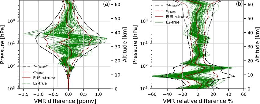
While SF DOF is a scalar quantity, both SF AK and
SF ERR, defined by Eqs. (10) and (11), respectively, are Af,ll
SF AKl = (10)
vertical profiles of pure numbers. SF AK represents an ex- max Ai,ll
i∈L2
pansion on the vertical dimension of SF DOF and, in particu-
lar, is calculated level by level as the ratio between the diag-
The SF ERR (Eq. 11) at a given level is the ratio between
onal elements of the AK matrix of the FUS product and the
the minimum total error of the L2 measurements that have
maximum of the corresponding elements of the AK matrices
been fused and the total error of the FUS product. A value
of the fusing L2 measurements.
of SF ERR larger than 1.0 means that at a specific level
A value of SF AK larger than 1.0 at a specific vertical
the error of the FUS product is smaller than that of all the
level (indicated by the index l) means that at that level the
individual products.
diagonal value of the AK matrix of the FUS product has a
larger value than that of all the individual products. As we min σtotal,i,l
have seen in Figs. 3 and 4, the increase of the AK diagonal i∈L2
SF ERR l = (11)
σf total,l
https://doi.org/10.5194/amt-14-2041-2021 Atmos. Meas. Tech., 14, 2041–2053, 20212050 N. Zoppetti et al.: Application of the CDF algorithm to GEO and LEO ozone profiles
ular, the peaks of their AK rows tend to not coincide with the
nominal vertical level of the row itself.
3.4 Statistical analysis on a coarse horizontal resolution
We have seen that starting from 79 781 L2 measure-
ments (Table 2), when a coincidence grid box with size
0.5◦ × 0.625◦ is used, the number of fused profiles is 1939
(Table 3), with a reduction of the data volume of more than a
factor 40.
Table 4 provides a summary of the number of fused pro-
files and the provenance of the L2 profiles that contribute to
them for a fusion grid resolution of 1◦ × 1◦ . In this case, the
total number of FUS products is 775, with a reduction of the
data volume of more than a factor 100.
The synergy factors SF DOF, SF AK and SF ERR, in this
case have also been considered, and the resulting figures
(similar to Figs. 6 and 7) are reported in the Supplement. In
Figure 6. Scatter plot of SF DOF as a function of the number of L2 summary, the greater number of fusing observations in each
measurements fused in each coincidence grid cell; different colours fusion cell produces a further improvement for both the ver-
represent different FUS types. tical resolution and the total error. This observation confirms
that the CDF method can be used with a wide range of grid
box sizes and data compressions and that the quality of the
products generally improves with larger cells. An upper limit
The SFs defined by Eqs. (10) and (11) provide a conserva- to the grid box size is caused by the coincidence error ampli-
tive comparison because the fused product is compared with tude, which increases with the geographical variability, de-
the L2 product that at that level has the largest diagonal value grading the quality of the fused product. The study of this
in its AK matrix and with the one that has the smallest total aspect will be of crucial importance if the CDF is to be ap-
error at the same level (generally, these are two distinct L2 plied to species with greater spatial and temporal variability
products). than ozone or in any cases with very large spatial and tempo-
Figure 7 shows the SF AK (Fig. 7a) and SF ERR ral domains.
(Fig. 7b) profiles for the 1939 FUS products considered in
Table 3. We have used different colours to denote the prove-
nance of the L2 data contributing to the fused products and 4 Conclusions
different symbol sizes to infer the number of L2 fusing mea-
surements (the larger the symbol size, the larger the number This paper presents a feasibility study of the CDF technique
of L2 fusing profiles). The significant improvement obtained applied to L2 products simulated according to the charac-
with the fused products is confirmed by Fig. 6. In Fig. 7, con- teristics of the atmospheric Sentinel missions. Despite the
sidering symbols of the same colour, the size (N) increases approximations that characterize the simulated L2 products
moving horizontally in the graph (same vertical level) from (technical specifications that are not exactly in line with the
left to right (SF increasing). This fact denotes that for each ones of the atmospherics Sentinels with no systematic errors
FUS type, SF increases with N. This is not in contradiction added), this analysis allows for the evaluation of the perfor-
with the fact that symbols with different colours (FUS types) mances of the CDF algorithm in a realistic scenario.
and different sizes (N) can share the same position (SF, verti- In particular, we show the application of CDF to a sin-
cal level) on the graph. Some SF AK values, both in the tro- gle cell with a size of 0.5◦ in latitude and 0.625◦ in longi-
posphere and in the middle to upper atmosphere are smaller tude in which more than 100 L2 products are fused. Results
than 1; in the troposphere, this happens in 20 cells out of show that the fused product is characterized by higher in-
1939 while in the middle to upper atmosphere this happens formation content, smaller errors and smaller residuals (i.e.
in almost 500 cells for two possible and sometimes simul- smaller anomalies from the true profiles) compared to indi-
taneous circumstances. The first circumstance occurs when vidual L2 products. The information content being, with its
the introduction of the coincidence error provokes a sensi- improvement of the vertical resolution, the most important
ble degradation of the quality of the FUS AK matrix. The achievement.
second circumstance occurs, for example, when one of the This analysis is then extended to a larger domain consist-
L2 products is characterized by a vertical resolution that is ing of 79 781 L2 products subdivided into 1939 grid boxes
much better than all the other fusing products and, in partic- of 0.5◦ × 0.625◦ size. In this case, the comparison of L2
Atmos. Meas. Tech., 14, 2041–2053, 2021 https://doi.org/10.5194/amt-14-2041-2021N. Zoppetti et al.: Application of the CDF algorithm to GEO and LEO ozone profiles 2051
Figure 7. (a) SF AK vs. vertical level. (b) SF ERR vs. vertical level. In both panels, the different colours of the symbols represent the FUS
type, and the different sizes of the symbols represent the number of measurements that have been fused. The maximum symbol size shown
in the legend corresponds to N = 160.
Table 4. Like in Table 2 but with a grid box size of 1◦ × 1◦ . Ncells is the number of grid boxes characterized by the considered FUS type.
< NL2 > is the mean number of individual L2 fusing profiles per grid box and maxNL2 is the maximum number of individual L2 fusing
products per grid box.
FUS type Description Ncells < NL2 > maxNL2
GEO:TIR + UV1 Two or more GEO pixels, no LEO pixels. 354 73.1 420
GEO:TIR + UV1_LEO:TIR + UV1 Two or more GEO pixels, one or more LEO-TIR pixel, 140 289.4 504
one or more LEO-UV1 pixel.
GEO:TIR + UV1_LEO:TIR Two or more GEO pixels, one or more GEO-TIR pixel, 79 115.4 442
no LEO-UV1 pixels.
GEO:TIR + UV1_LEO:UV1 Two or more GEO pixels, one or more LEO-UV1 pixel, 0 0 0
no LEO-TIR pixels.
LEO:TIR + UV1 No GEO pixels, one or more LEO-TIR pixels, 142 26.2 71
one or more LEO-UV1 pixels.
LEO:TIR No GEO pixels, two or more LEO-TIR pixels, 60 8.9 26
no LEO-UV1 pixels.
Total 775 102.9 504
products and CDF output are carried on in terms of syn- considered a new type of Level 3 product with improved
ergy factors. This analysis shows that the CDF can be ap- quality (reduced bias) and the same characteristics (AK in-
plied to a wide range of situations and that the benefits of cluded) with respect to L2 products, even if further analysis
the fusion strongly depend on the number of measurements is needed, especially concerning the coincidence error to be
that are fused and on their characteristics. It is also shown applied to fuse data on large spatial and temporal domains.
that CDF can be run by customizing grid resolutions, e.g. to
match the resolution requirements of the process that will in-
gest the products, with full exploitation of all the available Data availability. The data of the simulations presented in the pa-
measurements. per are available from the authors upon request.
As the fused products are traced back to a regular, fixed MERRA-2 data (atmospheric scenario) are available at https://
horizontal grid and, as shown here, are not affected by the gmao.gsfc.nasa.gov/reanalysis/MERRA-2/ (last access: 29 Decem-
ber 2020, NASA GMAO, 2020).
bias introduced by the a priori information, they can be
https://doi.org/10.5194/amt-14-2041-2021 Atmos. Meas. Tech., 14, 2041–2053, 20212052 N. Zoppetti et al.: Application of the CDF algorithm to GEO and LEO ozone profiles
The ML climatology is available at https://acd-ext.gsfc.nasa. References
gov/anonftp/toms/ML_climatology/ (last access: 17 February 2021,
NASA GSFC, 2021). The ML climatology is available as ASCII
tables of ozone mixing ratios (ML_ppmv_table.dat), the associ- Aires, F., Aznay, O., Prigent, C., Paul, M., and Bernardo, F.: Syner-
ated standard deviations (ML_ppmv_stats.dat), and a table of ozone gistic multi-wavelength remote sensing versus a posterior com-
layer amounts (ML_du_table.dat). bination of retrieved products: Application for the retrieval of
atmospheric profiles using MetOp-A, J. Geophys. Res., 117,
D18304, https://doi.org/10.1029/2011JD017188, 2012.
Supplement. The supplement related to this article is available on- AURORA consortium (Advanced Ultraviolet Radiation and Ozone
line at: https://doi.org/10.5194/amt-14-2041-2021-supplement. Retrieval for Applications, grant no. 687428): Technical Note
On L2 Data Simulations [D3.4], 35 pp., available at: https:
//cordis.europa.eu/project/id/687428/results (last access: 29 De-
cember 2020), 2017.
Author contributions. NZ wrote the Python code that implemented
Ceccherini, S., Carli, B., and Raspollini, P.: Equivalence of data fu-
the CDF, applied it to simulated data, collaborated with the study
sion and simultaneous retrieval, Opt. Express, 23, 8476–8488,
planning and the interpretation of the results, created all of the fig-
https://doi.org/10.1364/OE.23.008476, 2015.
ures, and wrote the paper’s draft version. SC deduced the CDF ex-
Ceccherini, S., Carli, B., Tirelli, C., Zoppetti, N., Del Bianco,
pressions, wrote the first version of the CDF code, and collaborated
S., Cortesi, U., Kujanpää, J., and Dragani, R.: Importance of
on the study planning and the interpretation of the results. FB main-
interpolation and coincidence errors in data fusion, Atmos.
tained and organized the calculus resources used for this work. BC
Meas. Tech., 11, 1009–1017, https://doi.org/10.5194/amt-11-
supervised the study, promoted the insights into the vertical resolu-
1009-2018, 2018.
tion, and collaborated on the study planning and the interpretation
Ceccherini, S., Zoppetti, N., Carli, B., Cortesi, U., Del Bianco,
of the results. RvdA led the work package regarding the simulation
S., and Tirelli, C.: The cost function of the data fusion pro-
of synthetic data. JCAvP generated the orbit data for all of the sim-
cess and its application, Atmos. Meas. Tech., 12, 2967–2977,
ulated L2 datasets. MG, CT, and SDB performed the simulation of
https://doi.org/10.5194/amt-12-2967-2019, 2019.
the infrared measurements. AA and JK performed the simulation of
Cortesi, U., Del Bianco, S., Ceccherini, S., Gai, M., Dinelli, B. M.,
the ultraviolet measurements. RD was responsible for choosing the
Castelli, E., Oelhaf, H., Woiwode, W., Höpfner, M., and Gerber,
atmospheric scenario and the ozone climatology. SdB and CT acted
D.: Synergy between middle infrared and millimeter-wave limb
in the role of project manager for the first and the second and third
sounding of atmospheric temperature and minor constituents, At-
year of AURORA, respectively. UC collaborated on the study plan-
mos. Meas. Tech., 9, 2267–2289, https://doi.org/10.5194/amt-9-
ning and was the principal investigator of the AURORA project. All
2267-2016, 2016.
of the authors revised the paper.
Cortesi, U., Ceccherini, S., Del Bianco, S., Gai, M., Tirelli, C.,
Zoppetti, N., Barbara, F., Bonazountas, M., Argyridis, A., Bós,
A., Loenen, E., Arola, A., Kujanpää, J., Lipponen, A., Nyamsi,
Competing interests. The authors declare that they have no conflict W. W., van der A, R., van Peet, J., Tuinder, O., Farruggia, V.,
of interest. Masini, A., Simeone, E., Dragani, R., Keppens, A., Lambert, J.-
C., van Roozendael, M., Lerot, C., Yu, H., and Verberne, K.:
Advanced Ultraviolet Radiation and Ozone Retrieval for Appli-
Acknowledgements. The results presented in this paper arise from cations (AURORA): A Project Overview, Atmosphere, 9, 454,
research activities conducted in the framework of the AURORA https://doi.org/10.3390/atmos9110454, 2018.
project (http://www.aurora-copernicus.eu/, last access: 29 Decem- Crevoisier, C., Clerbaux, C., Guidard, V., Phulpin, T., Armante,
ber 2020) supported by the Horizon 2020 research and innovation R., Barret, B., Camy-Peyret, C., Chaboureau, J.-P., Coheur, P.-
programme of the European Union (Call H2020-EO-2015; Topic F., Crépeau, L., Dufour, G., Labonnote, L., Lavanant, L., Hadji-
EO-2-2015) under grant agreement no. 687428. Lazaro, J., Herbin, H., Jacquinet-Husson, N., Payan, S., Péquig-
not, E., Pierangelo, C., Sellitto, P., and Stubenrauch, C.: Towards
IASI-New Generation (IASI-NG): impact of improved spectral
Financial support. This research has been supported by the Hori- resolution and radiometric noise on the retrieval of thermody-
zon 2020 research and innovation programme of the European namic, chemistry and climate variables, Atmos. Meas. Tech., 7,
Union (Call H2020-EO-2015; Topic EO-2-2015) under grant agree- 4367–4385, https://doi.org/10.5194/amt-7-4367-2014, 2014.
ment no. 687428, research activities conducted in the framework Cuesta, J., Eremenko, M., Liu, X., Dufour, G., Cai, Z., Höpfner,
of the AURORA project (http://www.aurora-copernicus.eu/, last ac- M., von Clarmann, T., Sellitto, P., Foret, G., Gaubert, B., Beek-
cess: 29 December 2020). mann, M., Orphal, J., Chance, K., Spurr, R., and Flaud, J.-M.:
Satellite observation of lowermost tropospheric ozone by mul-
tispectral synergism of IASI thermal infrared and GOME-2 ul-
Review statement. This paper was edited by Thomas von Clarmann traviolet measurements over Europe, Atmos. Chem. Phys., 13,
and reviewed by two anonymous referees. 9675–9693, https://doi.org/10.5194/acp-13-9675-2013, 2013.
ESA, Mission Science Division: GMES Sentinels 4 and 5 Mis-
sion Requirements Document (MRD), EOP-SM/2413, issue 1
rev. 0, available at: http://aurora.ifac.cnr.it/utils/personaldocs/
see/93/ (last access: 29 December 2020), 2011.
Atmos. Meas. Tech., 14, 2041–2053, 2021 https://doi.org/10.5194/amt-14-2041-2021N. Zoppetti et al.: Application of the CDF algorithm to GEO and LEO ozone profiles 2053 ESA, Mission Science Division: GMES Sentinels 4 and 5 Mis- NASA GSFC (Goddard Space Flight Center): Atmospheric Chem- sion Requirements Traceability Document (MRTD), EOP- istry and Dynamics Laboratory: McPeters and Labow Clima- SM/2413/BV-bv, issue 1 rev. 0, available at: http://aurora. tology, available at: https://acd-ext.gsfc.nasa.gov/anonftp/toms/ ifac.cnr.it/utils/personaldocs/see/96/ (last access: 29 December ML_climatology/, last access: 17 February 2021. 2020), 2012. Natraj, V., Liu, X., Kulawik, S., Chance, K., Chatfield, R., Edwards, EUMETSAT: MTG End-User Requirements Document, D. P., Eldering, A., Francis, G., Kurosu, T., Pickering, K., Spurr, EUM/MTG/SPE/07/0036, v3C, available at: https://www.ncdc. R., and Worden, H.: Multi-spectral sensitivity studies for the re- noaa.gov/sites/default/files/attachments/PDF_MTG_EURD.pdf trieval of tropospheric and lowermost tropospheric ozone from (last access: 29 December 2020), 2010. simulated clear-sky GEO-CAPE measurements, Atmos. Envi- Gelaro, R., McCarty, W., Max J. Suárez, M. J., Todling, R., Molod, ron., 45, 7151–7165, 2011 A., Takacs, L., Randles, C. A., Darmenov, A., Bosilovich, M. Ridolfi, M. and Sgheri, L.: A self-adapting and altitude-dependent G., Reichle, R., Wargan, K., Coy, L., Cullather, R., Draper, C., regularization method for atmospheric profile retrievals, Atmos. Akella, S., Buchard, V., Conaty, A., da Silva, A. M., Gu, W., Kim, Chem. Phys., 9, 1883–1897, https://doi.org/10.5194/acp-9-1883- G. K., Koster, R., Lucchesi, R., Merkova, D., Nielsen, J. E., Par- 2009, 2009. tyka, G., Pawson, S., Putman, W., Rienecker, M., Schubert, S. D., Rodgers, C. D.: Inverse Methods for Atmospheric Sounding: The- Sienkiewicz, M., and Zhao, B.: The Modern-Era Retrospective ory and Practice, Vol. 2 of Series on Atmospheric, Oceanic and Analysis for Research and Applications, Version 2 (MERRA-2), Planetary Physics, World Scientific, Singapore, 2000. J. Climate, 30, 5419–5454, https://doi.org/10.1175/JCLI-D-16- Sato, T. O., Sato, T. M., Sagawa, H., Noguchi, K., Saitoh, N., Irie, 0758.1, 2017. H., Kita, K., Mahani, M. E., Zettsu, K., Imasu, R., Hayashida, S., Lahoz, W. A. and Schneider, P.: Data assimilation: making sense and Kasai, Y.: Vertical profile of tropospheric ozone derived from of Earth Observation, Frontiers in Environmental Science, 2, 16, synergetic retrieval using three different wavelength ranges, UV, https://doi.org/10.3389/fenvs.2014.00016, 2014. IR, and microwave: sensitivity study for satellite observation, At- Liu, X., Bhartia, P. K., Chance, K., Spurr, R. J. D., and mos. Meas. Tech., 11, 1653–1668, https://doi.org/10.5194/amt- Kurosu, T. P.: Ozone profile retrievals from the Ozone Mon- 11-1653-2018, 2018. itoring Instrument, Atmos. Chem. Phys., 10, 2521–2537, Tirelli, C., Ceccherini, S., Zoppetti, N., Del Bianco, S., Gai, https://doi.org/10.5194/acp-10-2521-2010, 2010. M., Barbara, F., Cortesi, U., Kujanpää, J., Huan, Y., and Dra- McPeters, R. D. and Labow, G. J.: Climatology 2011: An gani, R.: Data fusion analysis of Sentinel-4 and Sentinel-5 MLS and sonde derived ozone climatology for satel- simulated ozone data, J. Atmos. Ocean. Tech., 37, 573–587, lite retrieval algorithms, J. Geophys. Res., 117, D10303, https://doi.org/10.1175/JTECH-D-19-0063.1, 2020. https://doi.org/10.1029/2011JD017006, 2012. von Clarmann, T. and Glatthor, N.: The application of mean Miles, G. M., Siddans, R., Kerridge, B. J., Latter, B. G., and averaging kernels to mean trace gas distributions, Atmos. Richards, N. A. D.: Tropospheric ozone and ozone profiles re- Meas. Tech., 12, 5155–5160, https://doi.org/10.5194/amt-12- trieved from GOME-2 and their validation, Atmos. Meas. Tech., 5155-2019, 2019. 8, 385–398, https://doi.org/10.5194/amt-8-385-2015, 2015. NASA GMAO (Global Modeling and Assimilation Office): Modern-Era Retrospective analysis for Research and Appli- cations, Version 2 (MERRA-2), NASA GES DISC, avail- able at: https://gmao.gsfc.nasa.gov/reanalysis/MERRA-2/, last access: 29 December 2020. https://doi.org/10.5194/amt-14-2041-2021 Atmos. Meas. Tech., 14, 2041–2053, 2021
You can also read