Bathymetric mapping of submarine sand waves using multiangle sun glitter imagery: a case of the Taiwan Banks with ASTER stereo imagery
←
→
Page content transcription
If your browser does not render page correctly, please read the page content below
Bathymetric mapping of submarine
                sand waves using multiangle sun
                glitter imagery: a case of the Taiwan
                Banks with ASTER stereo imagery

                Hua-guo Zhang
                Kang Yang
                Xiu-lin Lou
                Dong-ling Li
                Ai-qin Shi
                Bin Fu

Downloaded From: https://www.spiedigitallibrary.org/journals/Journal-of-Applied-Remote-Sensing on 14 Jul 2021
Terms of Use: https://www.spiedigitallibrary.org/terms-of-use
Bathymetric mapping of submarine sand waves using
                                  multiangle sun glitter imagery: a case of the Taiwan
                                          Banks with ASTER stereo imagery

                                              Hua-guo Zhang,* Kang Yang, Xiu-lin Lou, Dong-ling Li,
                                                             Ai-qin Shi, and Bin Fu
                                  Second Institute of Oceanography, State Key Laboratory of Satellite Ocean Environment
                                 Dynamics, State Oceanic Administration, No. 36 Baochubeilu Road, Hangzhou 310012, China

                                 Abstract. Submarine sand waves are visible in optical sun glitter remote sensing images and
                                 multiangle observations can provide valuable information. We present a method for bathymetric
                                 mapping of submarine sand waves using multiangle sun glitter information from Advanced
                                 Spaceborne Thermal Emission and Reflection Radiometer stereo imagery. Based on a multiangle
                                 image geometry model and a sun glitter radiance transfer model, sea surface roughness is derived
                                 using multiangle sun glitter images. These results are then used for water depth inversions based
                                 on the Alpers–Hennings model, supported by a few true depth data points (sounding data). Case
                                 study results show that the inversion and true depths match well, with high-correlation coeffi-
                                 cients and root-mean-square errors from 1.45 to 2.46 m, and relative errors from 5.48% to
                                 8.12%. The proposed method has some advantages over previous methods in that it requires
                                 fewer true depth data points, it does not require environmental parameters or knowledge of
                                 sand-wave morphology, and it is relatively simple to operate. On this basis, we conclude
                                 that this method is effective in mapping submarine sand waves and we anticipate that it will
                                 also be applicable to other similar topography types. © The Authors. Published by SPIE under a
                                 Creative Commons Attribution 3.0 Unported License. Distribution or reproduction of this work in
                                 whole or in part requires full attribution of the original publication, including its DOI. [DOI: 10
                                 .1117/1.JRS.9.095988]

                                 Keywords: multiangle; sun glitter remote sensing; submarine sand waves; bathymetric
                                 mapping.
                                 Paper 15213 received Mar. 19, 2015; accepted for publication Oct. 19, 2015; published online
                                 Nov. 16, 2015.

                                 1 Introduction
                                 Remote sensing of ocean bottom topography is an important research area that is significant for
                                 sea floor mapping and submarine object detection.1,2 Shallow water bathymetry features were
                                 first discovered on radar images in 1969.3,4 Since then, numerous studies have found that under
                                 low-to-moderate wind and strong tidal current conditions, real aperture radar and synthetic aper-
                                 ture radar (SAR) can detect bottom topography features in both shallow1,5–7 and deep waters.2
                                 One-dimensional (1-D) SAR imaging of shallow water bottom topography was first proposed by
                                 Alpers and Hennings,8 and a theoretical model was provided.8,9 Many researchers have sub-
                                 sequently studied ocean topography in SAR images worldwide. For example, Vogelzang
                                 et al.10,11 performed experiments to study the imaging of bottom topography with polarimetric
                                 P-, L-, and C-band SAR. Fu et al.12 studied SAR imaging mechanisms of sea bottom topography
                                 and analyzed the relationship between topographic parameters and SAR mapping of sea bottom
                                 topography. Yang et al.13 developed a detection model for underwater topography with a series of
                                 SAR images acquired at different times by combining the model with tide and tidal-current
                                 numerical simulations.

                                 *Address all correspondence to: Hua-guo Zhang, E-mail: zhanghg@163.com

                                 Journal of Applied Remote Sensing                      095988-1                        Vol. 9, 2015

Downloaded From: https://www.spiedigitallibrary.org/journals/Journal-of-Applied-Remote-Sensing on 14 Jul 2021
Terms of Use: https://www.spiedigitallibrary.org/terms-of-use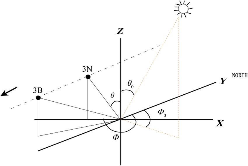
Zhang et al.: Bathymetric mapping of submarine sand waves using multiangle sun glitter imagery

                                     Sun glitter remote sensing is another remote sensing method based on variations in sea sur-
                                 face roughness (SSR). Cox and Munk14 developed the well-known mathematical relationship
                                 between sun glitter radiance and the probability distribution of the reflecting facets’ slope,
                                 allowing the surface to be observed (the Cox-Munk model). The Cox–Munk model established
                                 a fundamental theory enabling sun glitter images to detect marine dynamic processes, and sun
                                 glitter remote sensing has played an important role in a wide range of oceanographic studies,
                                 including internal wave detection,15,16 oil slick detection,17 and shallow underwater topography
                                 mapping.7,18 Hennings et al.19 developed a key theory of the sun glitter imaging mechanisms for
                                 underwater bottom topography based on the Cox-Munk model and SAR imaging mechanisms.
                                 He et al.,20 Shao et al.,21 and Zhang et al.22 used sun glitter imagery to observe sand waves in the
                                 Taiwan Banks, and statistically analyzed their distributions and characteristics. According to the
                                 sun glitter geometry model, it has been found that the signature of sun glitter images depends
                                 strongly on the viewing angle.19,23,24 He et al.25 discussed the brightness reversal of the Taiwan
                                 Banks submarine sand waves in sun glitter images from charge-coupled diodes onboard the
                                 HJ-1B satellite. Therefore, multiangle sun glitter images can present useful additional informa-
                                 tion compared with single angle images. Chust and Sagarminaga26 tested the use of the multi-
                                 angle imaging spectroradiometer (MISR) for detecting oil spills in Lake Maracaibo, and found
                                 that the MISR sensor has an improved capability for oil spill discrimination compared with the
                                 single-view moderate resolution imaging spectroRadiometer sensor. Matthews27 utilized the
                                 nadir and back-looking views of the Advanced Spaceborne Thermal Emission and
                                 Reflection Radiometer (ASTER) to detect internal waves and ship wakes, and he also proposed
                                 a “Back to Nadir” ratio to estimate SSR, In addition, he suggested that more information could
                                 be extracted from multiangle data. However, bathymetric mapping of submarine topography
                                 using multiangle sun glitter images has not yet been explored.
                                     In this paper, we present a method for bathymetric mapping of submarine sand waves using
                                 multiangle sun glitter imagery. The study area and data are introduced in the Sec. 1. Then, the
                                 methodology, including multiangle sun glitter geometry, a sun glitter image model, and a depth
                                 retrieval method are presented. Finally, a case study and its calculation results are discussed.

                                 2 Study Area and Data

                                 2.1 Study Area
                                 The study area is located in the Taiwan Banks, at the southern entrance of the Taiwan Strait. In
                                 this region, sand waves in shallow water shoals (namely, the Taiwan Banks) are characterized by
                                 large wave heights.28,29 Covering a total area of approximately 16;400 km2, the Taiwan Banks
                                 extend west–east (from Dongshan Island and the Fujian coast region to the Penghu Islands),22
                                 centered at 23°00’N, 118°30’E. Water depths in the Taiwan Banks are relatively shallow, ranging
                                 from 10 to 35 m, with an average depth of 20 m. Owing to the input of coastal sediments and
                                 nonferrous materials, the highest water optical transparency is only about 30 m, while in the
                                 nearshore, zone values range from just 2 to 10 m.30 Therefore, it is difficult for visible solar
                                 radiance to reach the marine bottom, making it particularly difficult to identify seafloor bathym-
                                 etry using remote sensing methods. However, the submarine sand waves are always visible using
                                 sun glitter images.31

                                 2.2 Satellite Imagery and Sounding Data
                                 ASTER is an advanced multispectral imager onboard the NASA’s Terra spacecraft that was
                                 launched in December 1999. The ASTER instrument consists of three separate instrument sub-
                                 systems: the visible and near-infrared (VNIR), the shortwave infrared, and the thermal infrared
                                 sensors. The VNIR sensor has three bands with a spatial resolution of 15 m, and an additional
                                 backward telescope for stereo observation. Channel 3N at nadir has the same bandwidth (0.78 to
                                 0.86 μm for near-infrared), and channel 3B has a back-looking view that detects the same region
                                 after 55 s. Initially, the stereo imaging mode was designed for the terrestrial sciences, e.g., for
                                 generating high-accuracy digital elevation models. However, for sun glitter investigations, the

                                 Journal of Applied Remote Sensing                     095988-2                              Vol. 9, 2015

Downloaded From: https://www.spiedigitallibrary.org/journals/Journal-of-Applied-Remote-Sensing on 14 Jul 2021
Terms of Use: https://www.spiedigitallibrary.org/terms-of-use
Zhang et al.: Bathymetric mapping of submarine sand waves using multiangle sun glitter imagery
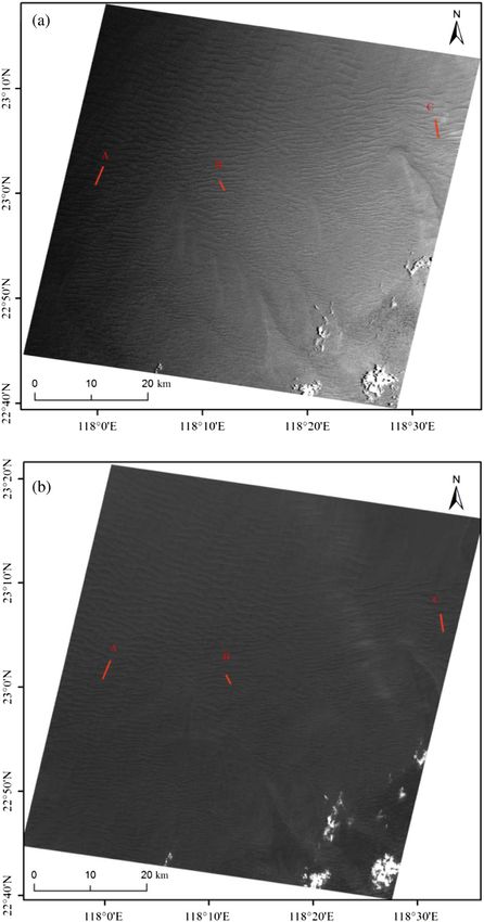
Fig. 1 Stereo images acquired on July 16, 2003, at 02:47:27 UTC by Advanced Spaceborne
Thermal Emission and Reflection Radiometer (ASTER) on board NASA’s Terra satellite.
(a) Nadir view image (NVI) and (b) back-looking view image (BVI). The red lines labeled A, B,
and C denote the profiles presented in Fig. 3.
Journal of Applied Remote Sensing 095988-3 Vol. 9, 2015
Downloaded From: https://www.spiedigitallibrary.org/journals/Journal-of-Applied-Remote-Sensing on 14 Jul 2021
Terms of Use: https://www.spiedigitallibrary.org/terms-of-useZhang et al.: Bathymetric mapping of submarine sand waves using multiangle sun glitter imagery
high spatial resolution (15 m), the sensor tilt capability, and the back-looking view from channel
3B, mean that ASTER has considerable potential for multiangle ocean remote sensing.
Figure 1(a) shows the nadir view image (NVI) imaged by channel 3N of the VNIR sensor in
the study area on July 16, 2003, at 02:47:27 UTC. Most of the sand waves are well-defined in the
high-quality image, with dark and bright strips clearly visible. However, the brightness of the
entire image increases from west to east, suggesting a matching tendency in the sun glitter radi-
ance. Figure 1(b) is the back-looking view image (BVI) gathered by channel 3B of the VNIR
sensor, obtained after 55 s for the same area. Relative to the NVI, the brightness of the BVI
descends smoothly over the entire image. The tidal flow-field of the sea surface was obtained
using a numerical calculation model. At the time the images were captured, the tidal flow direc-
tion, which was almost perpendicular to the sand-wave-crest orientation was from south to north
with speed of 0.824 ms−1 .
The bathymetric data used in this study was obtained by the R2Sonic 2024 broadband multi-
beam echo sounder device using the fifth generation multibeam architecture. The device can be
used in submarine bathymetry surveys in the range of 1 to 500 m. Its frequency range is from 200
to 400 kHz, selectable swath coverage is from 10 deg to 160 deg, beam angle is 0.5 deg ×1 deg
with 256 efficient beams, and resolution is 1.25 cm. The sounding data for this study was
obtained from May 25, 2012, to June 28, 2012, and has data spacing for two adjacent points
of 10 m.
3 Methodology
According to Hennings et al.,19 the mechanism of sun glitter imaging for bottom topography is
similar to that for SAR imaging described by Alpers and Hennings.8 The difference is that the
Bragg resonant scattering model is replaced by the Cox–Munk model14 to express variations in
the SSR shown by sun glitter images. The mechanism includes three processes:19 (1) interactions
between sea bottom topography and the current cause modulations in the surface current veloc-
ity; (2) modulations in the surface current cause variations in the spectrum of surface short waves
that determine the SSR; (3) variations in the SSR show in sun glitter images. However, the im-
aging geometry is a critical issue for stereo sun glitter remote sensing. Therefore, we first intro-
duce the stereo sun glitter geometry and develop a method for determining the imaging geometry
of each pixel. Then we introduce the mechanisms for modeling sun glitter imaging of submarine
sand waves. Finally, we present a new method for retrieving the water depth of sand waves using
the stereo sun glitter images.
3.1 Multiangle Sun Glitter Geometry
The header file of the ASTER image only provides two angles: the pointing angle (P) and the
scene orientation angle (S). However, previous researchers have generally used P and S to
identify the entire image. Matthews27 discusses sun glitter geometry in the nadir and back-
looking view ASTER images, but his calculation focuses on only one side of the nadir,
whereas angles may change when the ASTER image is acquired from both sides of the
nadir. Yang et al.32 provided an improved treatment of the sun glitter geometry of each
pixel in ASTER imagery. Figure 2 shows the observational geometry for sun glitter in
ASTER stereo image pairs.
The sun zenith angle (θ0 ) and the sun azimuth angle (∅0 ) of each pixel can be determined by
its position and imaging time. The view angle and the sensor zenith angle in the nadir view are θN
and ∅N , respectively, and the view angle and the sensor zenith angle in the back-looking view are
θB and ∅B , respectively.32 The view angle in the NVI is given by
θN ¼ n IFOV þ P;
EQ-TARGET;temp:intralink-;e001;116;140 (1)
where n denotes the pixel number from the sensor center, IFOV is instantaneous field of view,
and P denotes the pointing angle of the image.
Journal of Applied Remote Sensing 095988-4 Vol. 9, 2015
Downloaded From: https://www.spiedigitallibrary.org/journals/Journal-of-Applied-Remote-Sensing on 14 Jul 2021
Terms of Use: https://www.spiedigitallibrary.org/terms-of-useZhang et al.: Bathymetric mapping of submarine sand waves using multiangle sun glitter imagery
Fig. 2 Observational geometry of ASTER stereo image pairs (after Matthews27).
The sensor zenith angle in the nadir view is given by
270 þ S; left side of nadir
∅N ¼ ; (2)
90 þ S; right side of nadir
EQ-TARGET;temp:intralink-;e002;116;525
where S denotes the scene orientation angle of the image.
The view angle in the BVI becomes
"pffiffiffiffiffiffiffiffiffiffiffiffiffiffiffiffiffiffiffiffiffiffiffiffiffiffiffiffiffiffiffiffiffiffiffiffiffiffiffiffiffiffiffiffiffiffiffiffiffiffiffiffiffiffiffiffiffiffiffiffiffiffiffiffiffiffiffiffiffiffiffiffiffi#
−1 ðh tan P þ mnÞ2 þ ðh tan α∕ cos PÞ2
θB ¼ tan EQ-TARGET;temp:intralink-;e003;116;456 ; (3)
h
where h denotes the satellite height (m), m denotes the spatial resolution of the VNIR sensor
(15 m), and α denotes the angle between the nadir view and the back-looking view (27.6 deg for
the VNIR sensor).
We can obtain the sensor zenith angle in BVI (∅B ) as
270 − tan−1 ðG∕ tan θB Þ þ S ; left side of nadir
∅B ¼ ; (4)
90 − tan−1 ðG∕ tan θB Þ þ S; right side of nadir
EQ-TARGET;temp:intralink-;e004;116;357
where G is the base-to-height within the stereo image pair (0.6 for ASTER stereo images).
3.2 Sun Glitter Imaging Model
In this study, the absolute value of radiance is not considered because only the variation of the
reflectance caused by SSR is of interest. Therefore, normalized sun glitter radiance, Lg , given by
Gordon is adopted in this study.33
RðωÞ
Lg ¼ pðzx ; zy Þ: (5)
4 cos θ cos4 β
EQ-TARGET;temp:intralink-;e005;116;227
The angle of reflection is ω, β denotes the tilt angle of the wave facet, RðωÞ denotes the
Fresnel reflection coefficient; they are calculated from the sensor view angle (θ), the sensor
zenith angle (∅), the sun zenith angle (θ0 ), and the sun azimuth angle (∅0 ). pðzx ; zy Þ is the
probability density function (PDF) as functions of individual slope components zx and zy . In
this study, the isotropic PDF (independence with wind direction) is used according to the
Cox and Munk model,14 and it is given by
1 tan2 β
pðzx ; zy Þ ¼ pðβÞ ¼ exp − 2 ; (6)
πðσ 20 þ δσ 2 Þ σ 0 þ δσ 2
EQ-TARGET;temp:intralink-;e006;116;110
Journal of Applied Remote Sensing 095988-5 Vol. 9, 2015
Downloaded From: https://www.spiedigitallibrary.org/journals/Journal-of-Applied-Remote-Sensing on 14 Jul 2021
Terms of Use: https://www.spiedigitallibrary.org/terms-of-useZhang et al.: Bathymetric mapping of submarine sand waves using multiangle sun glitter imagery
where σ 20 þ δσ 2 denotes the SSR, σ 20 denotes the wind-generated SSR (background roughness),
and δσ 2 denotes the variation of SSR modulated by the interaction of current and bottom topog-
raphy. There are several empirical expressions of σ 20 as the function of wind speed, but the Cox–
Munk model was testified to have the best performance by Zhang and Wang.24 The variation of
SSR, δσ 2 , is given by
Zkc
δσ 2 ¼
EQ-TARGET;temp:intralink-;e007;116;675 kδEðkÞdk; (7)
k0
where k is the wave number of short gravity waves, k0 is the lower wave number limit that
produces sun glitter radiance modulation, and kc is the maximum wave number where the effect
of surface tension is negligible. According to Hennings et al.,19 k0 ¼ 4.024 m−1 , and
kc ¼ 366.583 m−1 . δEðkÞ denotes the modulation of the spectral energy density of waves
and is given by
4þγ ∂U
δEðkÞ ¼ − EðkÞ ; (8)
μ ∂x
EQ-TARGET;temp:intralink-;e008;116;558
where γ denotes the relationship between group velocity and phase velocity of short waves;
for gravity waves, γ ¼ 0.5. μ denotes the relaxation rate. According to Shao et al.,31 μ is
approximately 0.055 s−1 for the Taiwan Banks. EðkÞ denotes the spectral energy density
of waves, and ∂U∕∂x denotes the current velocity gradient. The spectral energy density
EðkÞ is given by
EQ-TARGET;temp:intralink-;e009;116;45 EðkÞ ¼ ap k−4 ;
5 (9)
where ap is the Phillips constant (0.004).
Inserting Eqs. (8) and (9) into Eq. (7) gives
Zkc
4 þ γ ap ∂U
δσ 2 ¼ − dk: (10)
μ k3 ∂x
EQ-TARGET;temp:intralink-;e010;116;398
k0
3.3 Depth Retrieval Method
In order to calculate the SSR (σ 20 þ δσ 2 ), we directly calculate the ratio of the glitter radiance in
the NVI to that in the BVI, based on Eqs. (5) and (6)
2
LgN RðωN Þ cos θB cos4 βB tan βB − tan2 βN
¼ exp ; (11)
LgB RðωB Þ cos θN cos4 βN σ 20 þ δσ 2
EQ-TARGET;temp:intralink-;e011;116;277
where LgN , θN , RðωN Þ, and βN denote the normalized sun glitter radiance, the view angle, the
Fresnel reflection coefficient, and the tilt angle of the wave facet, respectively, in the NVI, and
LgB , θB , RðωB Þ and βB denote these parameters in the BVI. The SSR is given by
LgN RðωB Þ cos θN cos4 βN 1
SSR ¼ Ln : (12)
LgB RðωN Þ cos θB cos4 βB tan βB − tan2 βN
2
EQ-TARGET;temp:intralink-;e012;116;195
Because σ 20 denotes the background roughness (wind-generated SSR), we consider that
σ 20 ¼ SSR:
EQ-TARGET;temp:intralink-;e013;116;129 (13)
Therefore, δσ 2 is calculated by
δσ 2 ¼ SSR − SSR:
EQ-TARGET;temp:intralink-;e014;116;85 (14)
Journal of Applied Remote Sensing 095988-6 Vol. 9, 2015
Downloaded From: https://www.spiedigitallibrary.org/journals/Journal-of-Applied-Remote-Sensing on 14 Jul 2021
Terms of Use: https://www.spiedigitallibrary.org/terms-of-useZhang et al.: Bathymetric mapping of submarine sand waves using multiangle sun glitter imagery
(a) NVI BVI SSR
24 0.07
20 0.06
Image pixel value
16 0.05
SSR
12 0.04
8 0.03
4 0.02
0 500 1000 1500 2000 2500 3000 3500
Distance (m)
(b) NVI BVI SSR
28 0.06
24
0.05
Image pixel value
20
SSR
16 0.04
12
0.03
8
4 0.02
0 200 400 600 800 1000 1200 1400
Distance (m)
(c) NVI BVI SSR
36 0.06
32
28 0.05
Image pixel value
24
SSR
20 0.04
16
12 0.03
8
4 0.02
0 500 1000 1500 2000 2500 3000
Distance (m)
Fig. 3 Profiles of image pixel values and estimated sea surface roughness (SSR) at: (a) site A,
(b) site B, and (c) site C (locations shown in Fig. 1). Blue curves denote the profiles of image pixel
values for NVIs, red curves denote the profiles of image pixel values for BVIs, and green curves
denote the SSR profiles.
Journal of Applied Remote Sensing 095988-7 Vol. 9, 2015
Downloaded From: https://www.spiedigitallibrary.org/journals/Journal-of-Applied-Remote-Sensing on 14 Jul 2021
Terms of Use: https://www.spiedigitallibrary.org/terms-of-useZhang et al.: Bathymetric mapping of submarine sand waves using multiangle sun glitter imagery
On this basis, we can obtain the variation of SSR (δσ 2 ) using stereo sun glitter images. To
simplify Eq. (10), we suppose that the constant Z is given by
Zkc
4 þ γ ap
Z¼ − dk: (15)
μ k3
EQ-TARGET;temp:intralink-;e015;116;711
k0
On the basis of Eqs. (10) and (15), the current velocity gradient is given by
∂U δσ 2
¼ : (16)
∂x
EQ-TARGET;temp:intralink-;e016;116;639
Z
Considering the current velocity along a transect perpendicular to a sand wave crest, it is
possible to calculate the current velocity of each pixel site (n) by the following integration
Zn
δσ 2t
Un ¼ U0 þ
EQ-TARGET;temp:intralink-;e017;116;571 dt: (17)
Z
1
According to the Alpers–Hennings model,8 a 1-D model is used to describe the relationship
between current velocity and water depth with the continuity equation
EQ-TARGET;temp:intralink-;e018;116;490 U0 · d0 ¼ U n · dn ; (18)
where U 0 , d0 , and dn are the mean (background) current velocity, the mean depth, and the local
depth in the x-direction perpendicular to submarine topography (e.g., the sand wave crest),
respectively. U 0 and d0 can be considered as constants for a sand wave. Therefore, if U0
and d0 are given or calculated using some true water depth data points, the water depth for
the whole sand wave can be retrieved. In addition, Z, given by Eq. (15), is not sufficiently accu-
rate because the parameters in Eq. (15), such as γ, μ, ap , k0 , and kc , are determined using approx-
imations. Therefore, U n is also not sufficiently accurate to give water depth. However, its relative
values and varying trends can be used to estimate the relative depth of sand waves. Therefore, U0
and d0 can be set at any reasonable values (1.2 m∕s and 20 m in this case, respectively) to
calculate the relative depth of sand waves. Then some known true depths (at least two points,
ideally one sited at the crest of the sand wave and another at the trough) are input to project the
water depth of the whole sand wave.
4 Results and Discussions
From Figs. 1(a) and 1(b), three sites, labeled A, B, and C from west to east, were selected for
water depth inversion. The profiles of image values (the pixel gray values) in the NVI and the
BVI are plotted in Fig. 3, which shows that the curve trends for the NVI are almost exactly
opposite to the BVI trends, indicating the brightness reversal due to the different view angles.
For site A, the image values vary from 15.5 to 23.3 in the NVI, and from 5.2 to 9.5 in the BVI.
Average values are 18.9 and 7.2 for the NVI and BVI, respectively. For site B, the average image
values increase to 22.4 in the NVI and 7.4 in the BVI, and the image values vary from 19.0 to
26.7, and from 6.0 to 9.5 in the NVI and BVI, respectively. For site C, the average image values
further increase to 28.3 in the NVI and 7.8 in the BVI, and the image values range from 23.3 to
34.5 in the NVI, and from 6.0 to 10.3 in the BVI. Thus, the average image values increase
significantly from west to east in the NVI, varying by c. 50% (from 18.9 to 28.3), implying
that the sand waves at the east site are more easily distinguished than those at the west site.
However, no significant variations are seen in the BVI results from the three sites.
The pixel gray values are converted to radiance values by a radiation conversion transfor-
mation using the radiation parameters in the header file of the ASTER image. Then the radiance
values and image geometric angles are input to calculate SSR for each pixel using Eq. (12). The
SSRs of the three sites are shown by the green curves in Fig. 3, and range from 0.0300 to 0.0609,
Journal of Applied Remote Sensing 095988-8 Vol. 9, 2015
Downloaded From: https://www.spiedigitallibrary.org/journals/Journal-of-Applied-Remote-Sensing on 14 Jul 2021
Terms of Use: https://www.spiedigitallibrary.org/terms-of-useZhang et al.: Bathymetric mapping of submarine sand waves using multiangle sun glitter imagery
-10
Retrieval depth Sounding depth (a)
-15 P2 P3 P5
Water depth (m)
-20
-25
P1
-30
P4
P6
-35
S1 S2 S3
-40
0 500 1000 1500 2000 2500 3000 3500
Distance (m)
-10 (b)
Retrieval depth Sounding depth
-15
P1 P3 P4
Water depth (m)
-20
-25
-30 P2 P5
-35
S1 S2 S3
-40
0 200 400 600 800 1000 1200 1400
Distance (m)
-10
Retrieval depth Sounding depth (c)
P3 P5
-15 P1
Water depth (m)
-20
-25
P4
P2
-30
-35 S1 S2 S3
-40
0 500 1000 1500 2000 2500 3000
Distance (m)
Fig. 4 Results of water depth inversions at: (a) site A, (b) site B, and (c) site C, (locations shown in
Fig. 1). Blue curves denote the retrieval depths, and red curves denote the sounding depths. Dashed
lines denote the separation lines dividing the profiles into S1, S2, and S3 according to the sand-wave
morphology for relative depth projections. Black arrows denote the true depth data points used to
project relative depth, and only the points in each division (S1, S2, or S3) are used for projections in
this division, except that P2 in (b) and (c) was used for both S1 and S2.
Journal of Applied Remote Sensing 095988-9 Vol. 9, 2015
Downloaded From: https://www.spiedigitallibrary.org/journals/Journal-of-Applied-Remote-Sensing on 14 Jul 2021
Terms of Use: https://www.spiedigitallibrary.org/terms-of-useZhang et al.: Bathymetric mapping of submarine sand waves using multiangle sun glitter imagery
-10
R 2 = 0.8800 (a)
-15 RSME = 2.39 m
Average depth = 31.17 m
Relative RSME = 7.67%
-20
Retrieval depth (m)
-25
-30
-35
-40
-40 -35 -30 -25 -20 -15 -10
-45
Sounding depth (m)
-10 (b)
R2= 0.8721
-15 RSME = 2.46 m
Average depth = 30.31 m
Relative RSME = 8.12%
Retrieval depth (m)
-20
-25
-30
-35
-40
-40 -35 -30 -25 -20 -15 -10
Sounding depth (m)
-10
(c)
R 2 = 0.9444
-15 RSME = 1.45 m
Average depth = 26.47 m
Relative RSME = 5.48%
Retrieval depth (m)
-20
-25
-30
-35
-40
-40 -35 -30 -25 -20 -15 -10
Sounding depth (m)
Fig. 5 Accuracy evaluation results for retrieval depth compared with sounding depth at: (a) site A,
(b) site B, and (c) site C.
Journal of Applied Remote Sensing 095988-10 Vol. 9, 2015
Downloaded From: https://www.spiedigitallibrary.org/journals/Journal-of-Applied-Remote-Sensing on 14 Jul 2021
Terms of Use: https://www.spiedigitallibrary.org/terms-of-useZhang et al.: Bathymetric mapping of submarine sand waves using multiangle sun glitter imagery
0.02996 to 0.0506, and 0.0282 to 0.0509 at sites A, B, and C, respectively. The average SSR
values are 0.0422, 0.0379, and 0.0367 for sites A to C, respectively. The variations seen in the
SSR trend are contrary to those in the NVI values. However, the variation rate is only c. 15% less
than that for the average image values in NVI (c. 50%). In addition, the SSR profiles show clearer
bright–dark stripes than both the NVI and the BVI, indicating that multiangle images are more
valuable than single angle images for bathymetric mapping.
With the proposed method, δσ 2 and relative depth are calculated in turn based on the SSR.
Five to six true depths from sounding datasets are then used to project the relative depth of each
site. Among them, two true depths are used for each sand wave, separated according to the sand-
wave morphology. The true depth data points are shown by arrows in Fig. 4, along with the
inversion depths of the three sites. The associated accuracy evaluation results are shown in
Fig. 5. The root-mean-square error (RMSE) and the correlation coefficient (R2 ) between the
inversion depths and the true depths are then calculated. The relative errors are also calculated
as the ratio of the RMSE to the average water depth. The results from site A show that trend
shapes of the inversion and the true depths match well [Fig. 4(a)], and their correlation co-
efficient is high (R2 ¼ 0.8800), although there are some significant differences in the details.
The RMSE is 2.39 m and the relative error is 7.67%. Results from site B [Fig. 4(b)] and site C
[Fig. 4(c)] both show good inversions with high correlation coefficients (R2 ¼ 0.8721 and
R2 ¼ 0.9444). The RMSE and relative error for site B are 2.46 m and 8.12%, respectively,
and 1.45 m and 5.48% for site C.
Although our results seem unconvincing compared with 30 cm results from the bathymetry
assessment system (BAS) presented by Calkoen et al.,34 the water depth in the BAS case study
was relatively low (c. 5 m) compared with the water depth (c. 31.0 m) in this study. Compared
with the BAS study, this approach requires fewer true depths, does not require supporting envi-
ronmental parameters, and the operation is relatively simple. Compared with results from He,20
our approach achieves a similar accuracy, but requires fewer true depths. Although Shao et al.21
presented an approach for mapping submarine sand waves that required only a few true depths,
their technique is based on prior knowledge of sand wave morphology. In contrast, our approach
requires no knowledge of the morphology, and the operation is simpler and does not involve an
iterative process. In summary, the advantages of our proposed method include the requirement
for fewer true depths, the fact that supporting environmental parameters and knowledge of the
sand-wave morphology are not needed, and simpler operation. From the above analysis, given
the acceptable accuracies, we conclude that this approach represents a significant improvement
over previous methods. However, one limitation is that at least two view angle images simulta-
neously have distinguishable sun glitter information at the same time.
5 Conclusions
In this paper, we present a new method for bathymetric mapping of submarine sand waves using
stereo sun glitter images from the ASTER sensor. The results of our study yield a number of
important conclusions as follows.
Based on a multiangle image geometry model and a sun glitter radiance transfer model, a
method for deriving SSR was developed using multiangle sun glitter images. Compared with
methods that use single angle sun glitter data, our method avoids the dependence on observa-
tion angle.
A water depth inversion method was developed based on the Alpers–Hennings model, with a
few supporting true depth data points. The case study results show that the shapes of the trends
for the inversion and the true depths (sounding data) are well matched, and their correlation
coefficients are high (R2 ¼ 0.8800, R2 ¼ 0.8721, and R2 ¼ 0.9444). The accuracy evaluation
shows that the RMSE values range from 1.45 to 2.46 m, and that the relative errors range from
5.48% to 8.12%. Compared with previous research, our proposed method has equal or higher
precision with several some advantages. The proposed method requires fewer true depth data,
has no requirement for supporting environmental parameters or knowledge of sand-wave mor-
phology, and is relatively simple to operate. Given the acceptable accuracies, we conclude that
this approach represents a significant improvement over previous methods.
Journal of Applied Remote Sensing 095988-11 Vol. 9, 2015
Downloaded From: https://www.spiedigitallibrary.org/journals/Journal-of-Applied-Remote-Sensing on 14 Jul 2021
Terms of Use: https://www.spiedigitallibrary.org/terms-of-useZhang et al.: Bathymetric mapping of submarine sand waves using multiangle sun glitter imagery
We have shown that our method is effective in mapping submarine sand waves. It is also
anticipated that this method can be used to map other types of submarine topography because the
method is independent of terrain morphology. We consider that this method has significant
potential in the observation of submarine topography, particularly with the operation of an
increasing number of multiangle optical remote sensors. However, a limitation lies in that at
least two view angle images simultaneously have distinguishable sun glitter information. We
will conduct more case studies and improve the method.
Acknowledgments
The stereo-optical images used in this study were provided by the Center for Earth Observation
and Digital Earth, Chinese Academy of Sciences, China. The bathymetry data used in this study
were obtained under the Public Science and Technology Research Fund Project of Ocean (Grant
Number 201105001), and were processed by the Third Institute of Oceanography, State Oceanic
Administration, China. This research was supported by the Project of State Key Laboratory of
Satellite Ocean Environment Dynamics, Second Institute of Oceanography (Grant
Number SOEDZZ1513), the Public Science and Technology Research Fund Project of
Surveying, Mapping and Geoinformation (Grant Number 201512030), and the Public Science
and Technology Research Fund Project of Ocean (Grant Number 201105001). The authors
would like to thank Editage for English language editing.
References
1. W. Alpers et al., “Underwater topography,” in Synthetic Aperture Radar Marine User’s
Manual, C. R. Jackson and J. R. Apel, Eds., pp. 245–262, US Department of Commerce,
National Oceanic and Atmospheric Administration, National Environmental Satellite,
Data, and Information Serve, Office of Research and Applications, Washington DC (2004).
2. X. F. Li et al., “Deep-water bathymetric features imaged by spaceborne SAR in the Gulf
stream region,” Geophys. Res. Lett. 37, L19603 (2010).
3. G. P. De Loor, “Microwave measurements over the North Sea,” Boundary Layer Meteorol.
13(1–4), 119–131 (1978).
4. G. P. De Loor, “The observation of tidal patterns, currents, and bathymetry with SLAR
imagery of the sea,” IEEE J. Oceanic Eng. 6(4), 124–129 (1981).
5. X. F. Li et al., “Sea surface manifestation of along-tidal-channel underwater ridges imaged
by SAR,” IEEE Trans. Geosci. Remote Sens. 47(8), 2467–2477 (2009).
6. D. W. S. Lodge, “Surface expression of bathymetry on SEASAT synthetic aperture radar
images,” Int. J. Remote Sens. 4(3), 639–653 (1983).
7. W. Shi et al., “Ocean sand ridge signatures in the bohai sea observed by satellite ocean color and
synthetic aperture radar measurements,” Remote Sens. Environ. 115(8), 1926–1934 (2011).
8. W. Alpers and I. Hennings, “A theory of the imaging mechanism of underwater bottom
topography by real and synthetic aperture radar,” J. Geophys. Res. 89, 10529–10546 (1984).
9. R. A. Shuchman et al., “Synthetic aperture radar imaging of ocean-bottom topography via
tidal-current interactions: theory and observations,” Int. J. Remote Sens. 6(7), 1179–1200
(1985).
10. J. Vogelzang et al., “Sea bottom topography with polarimetric P-, L- and C- band SAR,” in
Remote Sensing Science for the Nineties, 10th Annual Int. Geoscience and Remote Sensing
Symp., 1990 (IGARSS’90), pp. 2467–2470, IEEE (1990).
11. J. Vogelzang et al., “Mapping submarine sand waves with multiband imaging radar: exper-
imental results and model comparison,” J. Geophys. Res. Oceans 102, 1183–1192 (1997).
12. B. Fu et al., “Simulation study of sea bottom topography mapping by spaceborne
SAR-Relationship between topographic parameters and measurement of water depth,”
Acta Oceanol. Sin. 23(1), 35–42 (2001).
13. J. G. Yang et al., “A detection model of underwater topography with a series of SAR images
acquired at different time,” Acta Oceanol. Sin. 29(4), 28–37 (2010).
14. C. Cox and W. Munk, “Measurement of the roughness of the sea surface from photographs
of the sun’s glitter,” J. Opt. Soc. Am. 44(11), 838–850 (1954).
Journal of Applied Remote Sensing 095988-12 Vol. 9, 2015
Downloaded From: https://www.spiedigitallibrary.org/journals/Journal-of-Applied-Remote-Sensing on 14 Jul 2021
Terms of Use: https://www.spiedigitallibrary.org/terms-of-useZhang et al.: Bathymetric mapping of submarine sand waves using multiangle sun glitter imagery
15. C. Jackson, “Internal wave detection using the moderate resolution imaging spectroradiom-
eter (MODIS),” J. Geophys. Res. Oceans 112(C11), C11012 (2007).
16. B. Liu et al., “Tracking the internal waves in the South China Sea with environmental
satellite sun glint images,” Remote Sens. Lett. 5(7), 609–618 (2014).
17. C. M. Hu et al., “Detection of natural oil slicks in the NW Gulf of Mexico using MODIS
imagery,” Geophys. Res. Lett. 36, L10604 (2009).
18. I. Hennings et al., “Comparison of submarine relief features on a radar satellite image and on
a Skylab satellite photograph,” Int. J. Remote Sens. 9(1), 45–67 (1988).
19. I. Hennings et al., “Sun glitter radiance and radar cross-section modulations of the sea bed,”
J. Geophys. Res. 99(C8), 16303–16326 (1994).
20. X. K. He, “Reconstruction of sand wave bathymetry using both satellite imagery and multi-
beam bathymetric data: a case study of the Taiwan Banks,” Int. J. Remote Sens. 35(9),
3286–3299 (2014).
21. H. Shao et al., “Priori knowledge based a bathymetry assessment method using the sun
glitter imagery: a case study of sand waves on the Taiwan Banks,” Acta Oceanol. Sin.
33(1), 120–126 (2014).
22. H. G. Zhang et al., “Observation of sand waves in the Taiwan Banks using HJ-1A/1B sun
glitter imagery,” J. Appl. Remote Sens. 8(1), 083570 (2014).
23. C. R. Jackson et al., “The role of the critical angle in brightness reversals on sunglint images
of the sea surface,” J. Geophys. Res. 115(C9), C09019 (2010).
24. H. Zhang and M. H. Wang, “Evaluation of sun glint models using MODIS measurements,”
J. Quant. Spectrosc. Radiat. Transfer 111, 492–506 (2010).
25. X. K. He et al., “The brightness reversal of submarine sand waves in ‘HJ-1A/B’ CCD sun
glitter images,” Acta Oceanolog. Sin. 34(1), 94–99 (2015).
26. G. Chust and Y. Sagarminaga, “The multi-angle view of MISR detects oil slicks under sun
glitter conditions,” Remote Sens. Environ. 107(1), 232–239 (2007).
27. J. Matthews, “Stereo observation of lakes and coastal zones using ASTER imagery,”
Remote Sens. Environ. 99(1), 16–30 (2005).
28. S. Boggs, “Sand-wave fields in Taiwan Strait,” Geology 2, 251–253 (1974).
29. Z. C. Liu et al., “The development in the latest technique of shallow water multi-beam
sounding system,” Hydrographic Surv. Charting 25, 67–70 (2005).
30. F. L. Li, “Annual variations of Secchi depth in the near shore waters of the western Taiwan
Strait during the summers of 1998–2010,” J. Oceanogr. Taiwan Strait 31(3), 301–306
(2012).
31. H. Shao et al., “Sun glitter imaging of submarine sand waves on the Taiwan Banks: deter-
mination of the relaxation rate of short waves,” J. Geophys. Res. 116(C6), C06024 (2011).
32. K. Yang et al., “Observation of submarine sand waves using ASTER stereo sun glitter
imagery,” Int. J. Remote Sens. (2015).
33. H. R. Gordon, “Atmospheric correction of ocean color imagery in the earth observing sys-
tem era,” J. Geophys. Res. 102(D14), 17081–17106 (1997).
34. C. J. Calkoen et al., “The bathymetry assessment system: efficient depth mapping in shallow
seas using radar images,” Int. J. Remote Sens. 22(15), 2973–2998 (2001).
Hua-guo Zhang is an associate professor of the Second Institute of Oceanography, State
Oceanic Administration, China. His research interest is the coastal remote sensing. He has pub-
lished more than 20 papers. He received his BS degree in environment from Nankai University in
1999, his MS degree in oceanography at the Second Institute of Oceanography, State Oceanic
Administration in 2002, and his PhD in oceanography from Ocean University of China in 2011.
Biographies for the other authors are not available.
Journal of Applied Remote Sensing 095988-13 Vol. 9, 2015
Downloaded From: https://www.spiedigitallibrary.org/journals/Journal-of-Applied-Remote-Sensing on 14 Jul 2021
Terms of Use: https://www.spiedigitallibrary.org/terms-of-useYou can also read