BERT Knows Punta Cana is not just beautiful, it's gorgeous: Ranking Scalar Adjectives with Contextualised Representations
←
→
Page content transcription
If your browser does not render page correctly, please read the page content below
BERT Knows Punta Cana is not just beautiful, it’s gorgeous:
       Ranking Scalar Adjectives with Contextualised Representations

                    Aina Garı́ Soler                            Marianna Apidianaki
                 Université Paris-Saclay                   Department of Digital Humanities
                     CNRS, LIMSI                                 University of Helsinki
                  91400 Orsay, France                              Helsinki, Finland
                aina.gari@limsi.fr                      marianna.apidianaki@helsinki.fi

                      Abstract
    Adjectives like pretty, beautiful and gorgeous
    describe positive properties of the nouns they
    modify but with different intensity. These dif-
    ferences are important for natural language
    understanding and reasoning. We propose a               Figure 1: Full scale of adjectives describing positive
    novel BERT-based approach to intensity de-              and negative sentiment at different degrees from the
    tection for scalar adjectives. We model inten-          SO-CAL dataset (Taboada et al., 2011).
    sity by vectors directly derived from contextu-
    alised representations and show they can suc-
    cessfully rank scalar adjectives. We evaluate           notion of adjective intensity. In what follows, we
    our models both intrinsically, on gold standard         explore this hypothesis using representations ex-
    datasets, and on an Indirect Question Answer-
                                                            tracted from different layers of this deep neural
    ing task. Our results demonstrate that BERT
    encodes rich knowledge about the semantics              model. Since the scalar relationship between adjec-
    of scalar adjectives, and is able to provide bet-       tives is context-dependent (Kennedy and McNally,
    ter quality intensity rankings than static em-          2005) (e.g., what counts as tall may vary from
    beddings and previous models with access to             context to context), we consider the contextualised
    dedicated resources.                                    representations produced by BERT to be a good fit
                                                            for this task. We also propose a method inspired by
1   Introduction                                            gender bias work (Bolukbasi et al., 2016; Dev and
Scalar adjectives describe a property of a noun at          Phillips, 2019) for detecting the intensity relation-
different degrees of intensity. Identifying the scalar      ship of two adjectives on the fly. We view intensity
relationship that exists between their meaning (for         as a direction in the semantic space which, once
example, the increasing intensity between pretty,           identified, can serve to determine the intensity of
beautiful and gorgeous) is useful for text under-           new adjectives.
standing, for both humans and automatic systems.               Our work falls in the neural network interpre-
It can serve to define the sentiment and subjectiv-         tation paradigm which explores the knowledge
ity of a text, perform inference and textual entail-        about language encoded in the representations of
ment (Van Tiel et al., 2016; McNally, 2016), build          deep learning models (Voita et al., 2019a; Clark
question answering and recommendation systems               et al., 2019; Voita et al., 2019b; Tenney et al., 2019;
(de Marneffe et al., 2010), and assist language learn-      Talmor et al., 2019). The bulk of this interpreta-
ers in distinguishing between semantically similar          tion work addresses structural aspects of language
words (Sheinman and Tokunaga, 2009).                        such as syntax, word order, or number agreement
   We investigate the knowledge that the pre-               (Linzen et al., 2016; Hewitt and Manning, 2019;
trained BERT model (Devlin et al., 2019) encodes            Hewitt and Liang, 2019; Rogers et al., 2020); shal-
about the intensity expressed on an adjective scale.        low semantic phenomena closely related to syn-
Given that this property is acquired by humans              tax such as semantic role labelling and corefer-
during language learning, we expect a language              ence (Tenney et al., 2019; Kovaleva et al., 2019);
model (LM) exposed to massive amounts of text               or the symbolic reasoning potential of language
data during training to have also acquired some             model representations (Talmor et al., 2019). Our

                                                        7371
      Proceedings of the 2020 Conference on Empirical Methods in Natural Language Processing, pages 7371–7385,
                       November 16–20, 2020. c 2020 Association for Computational Linguistics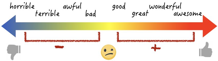
work makes a contribution towards the study of           larity (positive or negative) and intensity. Such
the knowledge pre-trained LMs encode about word          resources can be manually created, like the SO-
meaning, generally overlooked until now in inter-        CAL lexicon (Taboada et al., 2011), or automati-
pretation work.                                          cally compiled by mining adjective orderings from
   We evaluate the representations generated by          star-valued product reviews where people’s com-
BERT against gold standard adjective intensity esti-     ments have associated ratings (de Marneffe et al.,
mates (de Melo and Bansal, 2013; Wilkinson, 2017;        2010; Rill et al., 2012; Sharma et al., 2015; Rup-
Cocos et al., 2018) and apply them directly to a         penhofer et al., 2014). Cocos et al. (2018) com-
question answering task (de Marneffe et al., 2010).      bine knowledge from lexico-syntactic patterns and
Our results show that BERT clearly encodes the           the SO-CAL lexicon with paraphrases in the Para-
intensity variation between adjectives on scales de-     phrase Database (PPDB) (Ganitkevitch et al., 2013;
scribing different properties. Our proposed method       Pavlick et al., 2015).
can be easily applied to new datasets and languages         Our approach is novel in that it does not need
where scalar adjective resources are not available.1     specified patterns or access to lexicographic re-
                                                         sources. It, instead, relies on the knowledge about
2   Related Work                                         intensity encoded in scalar adjectives’ contextu-
                                                         alised representations. Our best performing method
The analysis of scalar adjective relationships in
                                                         is inspired by work on gender bias which relies on
the literature has often been decomposed into two
                                                         simple vector arithmetic to uncover gender-related
steps: Grouping related adjectives together and
                                                         stereotypes. A gender direction is determined (for
ranking adjectives in the same group according to
                                                         example, by comparing the embeddings of she and
intensity. The first step can be performed by dis-
                                                         he, or woman and man) and the projection of the
tributional clustering approaches (Hatzivassiloglou
                                                         vector of a potentially biased word on this direction
and McKeown, 1993; Pang et al., 2008) which can
                                                         is then calculated (Bolukbasi et al., 2016; Zhao
also address adjectival polysemy. Hot, for example,
                                                         et al., 2018). We extend this method to scalar ad-
can be on the TEMPERATURE scale (a warm → hot
                                                         jectives and BERT representations.
→ scalding drink), the ATTRACTIVENESS (a pretty
                                                            Kim and de Marneffe (2013) also consider vec-
→ hot → sexy person) or the INTEREST scale (an
                                                         tor distance in the semantic space to encode scalar
interesting → hot topic), depending on the attribute
                                                         relationships between adjectives. They specifically
it modifies.
                                                         examine a small set of word pairs, and observe that
   Other works (Sheinman and Tokunaga, 2009;
                                                         the middle point in space between the word2vec
de Melo and Bansal, 2013; Wilkinson, 2017) di-
                                                         (Mikolov et al., 2013) embeddings of two antonyms
rectly address the second step, ranking groups of
                                                         (e.g., furious and happy) falls close to the embed-
semantically related adjectives from lexicographic
                                                         ding of a mid-ranked word in their scale (e.g., un-
resources (e.g., WordNet) (Fellbaum, 1998). This
                                                         happy). Their experiments rely on antonym pairs
ranking is the focus of this work. We show that
                                                         extracted from WordNet. We show that contextu-
BERT contextualised representations encode rich
                                                         alised representations are a better fit for this task
information about adjective intensity, and can pro-
                                                         than static embeddings, encoding rich information
vide high quality rankings of adjectives in a scale.
                                                         about adjectives’ meaning and intensity.
   Adjective ranking has been traditionally per-
formed using pattern-based approaches which ex-          3       Data
tract lexical or syntactic patterns indicative of an
intensity relationship from large corpora (Shein-        We experiment with three scalar adjective datasets.
man and Tokunaga, 2009; de Melo and Bansal,
2013; Sheinman et al., 2013; Shivade et al., 2015).      DE M ELO     (de Melo and Bansal, 2013).2 Adjec-
For example, the patterns “X, but not Y” and “not        tive sets were extracted from WordNet ‘dumbbell’
just X but Y” provide evidence that X is an adjec-       structures (Gross and Miller, 1990). The sets rep-
tive less intense than Y. Another common approach        resent full-scales (e.g., from horrible to awesome)
is lexicon-based and draws upon a resource that          and are partitioned into half-scales (from horri-
maps adjectives to scores encoding sentiment po-         ble to bad, and from good to awesome) based on
                                                         pattern-based evidence in the Google N-Grams cor-
  1
    Our code and data are available at https://github.
                                                             2
com/ainagari/scalar_adjs                                         http://demelo.org/gdm/intensity/

                                                    7372
Dataset      Adjective scale                          2009)5 and the Flickr 30K dataset (Young et al.,
                     [soft → quiet → inaudible → silent]      2014).6 For every s ∈ D, a dataset from Section
        DE M ELO
                     [thick → dense → impenetrable]           3, and for each a ∈ s, we collect 1,000 instances
                     [fine → remarkable → spectacular]        (sentences) from each corpus.7 We substitute each
        C ROWD
                     [scary || frightening → terrifying]      instance i of a ∈ s, with each b ∈ s where b 6= a,
                     [damp → moist → wet]                     creating |s| − 1 new sentences.8 For example, for
        W ILKINSON
                     [dumb → stupid → idiotic]                an instance of thick from the scale [thick → dense
                                                              → impenetrable] in Table 1, we generate two new
Table 1: Examples of scales in each dataset. ‘||’ de-         sentences where thick is substituted by each of the
notes a tie between adjectives of the same intensity.         other adjectives in the same context.

                                                              4.2     Sentence Cleaning
pus (Brants and Franz, 2006). The dataset contains            Hearst patterns We filter out sentences where
87 half-scales with 548 adjective pairs, manually             substitution should not take place, such as cases
annotated for intensity relations (, and =).              of specialisation or instantiation. In this way, we
C ROWD (Cocos et al., 2018).3 The dataset consists            avoid replacing deceptive with fraudulent and false
of a set of adjective scales with high coverage of            in sentences like “Viruses and other deceptive soft-
the PPDB vocabulary. It was constructed by a three-           ware”, “Deceptive software such as viruses”, “De-
step process: Crowd workers were first asked to               ceptive software, especially viruses”.9 We parse
determine whether pairs of adjectives describe the            the sentences with stanza (Qi et al., 2020) to
same attribute (e.g., TEMPERATURE) and should,                reveal their dependency structure, and use Hearst
therefore, belong to the same scale. Sets of same-            lexico-syntactic patterns (Hearst, 1992) to iden-
scale adjectives were then refined over multiple              tify sentences describing is-a relationships between
rounds. Finally, workers ranked the adjectives in             nouns in a text. More details about this filtering are
each set by intensity. The final dataset includes 330         given in Appendix A.
adjective pairs along 79 half-scales.
                                                              Language Modelling criteria Adjectives that
W ILKINSON (Wilkinson and Oates, 2016).4 This                 belong to the same scale might not be replaceable
dataset was generated through crowdsourcing.                  in all contexts. Polysemy can also influence their
Crowd workers were presented with small seed sets             substitutability (e.g., warm weather is a bit hot, but
(e.g., huge, small, microscopic) and were asked to            a warm smile is friendly). In order to select contexts
propose similar adjectives, resulting in twelve ad-           where ∀a ∈ s fit, we measure the fluency of the
jective sets. Sets were automatically cleaned for             sentences generated through substitution. We use
consistency, and then annotated for intensity by the          a score assigned to each sentence by context2vec
crowd workers. The original dataset contains full             (Melamud et al., 2016) which reflects how well
scales. We use its division in 21 half-scales (with           an a ∈ s fits a context by measuring the cosine
61 adjective pairs) proposed by Cocos et al. (2018).          similarity between a and the context representa-
   In the rest of the paper, we use the term “scale” to       tion. We also experimented with calculating the
refer to the half-scales contained in these datasets.
                                                                  5
Table 1 shows examples from each one of them.                       http://u.cs.biu.ac.il/˜nlp/resources/
                                                              downloads/context2vec/
                                                                  6
                                                                    Flickr contains crowdsourced captions for 31,783 images
4       BERT Contextualised Representations                   describing everyday activities, events and scenes. We consider
                                                              objective descriptions to be a better fit for our task than subjec-
4.1       Sentence Collection                                 tive statements, which might contain emphatic markers. For
                                                              example, impossible would be a bad substitute for impractical
To explore the knowledge BERT has about rela-                 in the sentence “What you ask for is too impractical”.
                                                                  7
tionships in an adjective scale s, we generate a                    ukWaC has perfect coverage. Flickr 30K covers 96.56%
                                                              of the DE M ELO scales and 86.08% of the C ROWD scales. A
contextualised representation for each a ∈ s in the           scale s is not covered when no a ∈ s is found in a corpus.
                                                                  8
same context. Since such cases are rare in running                  We make a minor adjustment of the substituted data by
text, we construct two sentence sets that satisfy this        replacing the indefinite article a with an when the adjective
                                                              that follows starts with a vowel, and the inverse when it starts
condition using the ukWaC corpus (Baroni et al.,              with a consonant.
                                                                  9
                                                                    This would especially be a problem when considering
    3
        https://github.com/acocos/scalar-adj                  adjectives with different polarity on a full scale (e.g., deceptive
    4
        https://github.com/Coral-Lab/scales                   and honest).

                                                           7373
perplexity assigned by BERT to a sentence gener- Dataset Metric B ERT S IM FREQ SENSE
ated through substitution, and with replacing the P - ACC 0.59111 0.571 0.493
DE M ELO τ 0.36411 0.304 0.192
original a instance with the [MASK] token and get-
ρavg 0.38911 0.309 0.211
ting the BERT probability for each a ∈ s as a filler
P - ACC 0.64611 0.608 0.570
for that slot. context2vec was found to make better C ROWD τ 0.49811 0.404 0.428
substitutability estimates.10 ρavg 0.49411 0.499 0.537
We use a 600-dimensional context2vec model P - ACC 0.9139 0.7399 0.7399
in our experiments, pre-trained on ukWaC.11 We W ILKINSON τ 0.8269 0.478 0.586
calculate the context2vec score for all sentences ρavg 0.7249 0.345 0.493
generated for a scale s through substitution, and
Table 2: B ERT S IM results on each dataset using con-
keep the ten with the lowest standard deviation
textualised representations from the ukWaC SENT- SET.
(STD). Low STD for a sentence means that ∀a ∈ s Subscripts denote the best-performing BERT layer.
are reasonable choices in this context. For compar-
ison, we also randomly sample ten sentences from
all the ukWaC sentences collected for each scale.
We call the sets of sentences ukWaC, Flickr and
Random SENT- SETs.
We extract the contextualised representation for
each a ∈ s in the ten sentences retained for scale
s, using the pre-trained bert-base-uncased
model.12 This results in |s| ∗ 10 BERT represen-
tations for each scale. We repeat the procedure
for every BERT layer. Examples of the obtained
sentences are given in Appendix B.
5 Scalar Adjectives Ranking
5.1 Ranking with a Reference Point
Figure 2: Examples of B ERT S IM ranking predictions
In our first ranking experiment, we explore whether across layers using ukWaC sentences for four adjective
BERT encodes adjective intensity relative to a ref- scales: (a) [big → large → enormous → huge → gi-
erence point, that is the adjective with the highest gantic], (b) [good → great → wonderful → awesome],
intensity (aext ) in a scale s. (c) [cute → pretty → lovely → lovelier → breathtak-
ing], (d) [pleased → happy → excited → delighted →
Method We rank ∀a ∈ s where a 6= aext by overwhelmed]. (a) and (b) are from W ILKINSON, (c)
intensity by measuring the cosine similarity be- and (d) are from C ROWD.
tween their representation and that of aext in the
ten ukWaC sentences retained for s, and in every
BERT layer. For example, to rank [pretty, beau- dard ranking in the corresponding dataset D using
tiful, gorgeous] we measure the similarity of the Kendall’s τ and Spearman’s ρ correlation coeffi-
representations of pretty and beautiful to that of gor- cients.13 We also measure the model’s pairwise
geous. We then average the similarities obtained accuracy (P - ACC) which shows whether it correctly
for each a and use these values for ranking. We predicted the relative intensity (, =) for each
refer to this method as B ERT S IM. pair ai -aj ∈ s with i 6= j. During evaluation, we
We evaluate the quality of the ranking for a scale do not take into account scales where only one
by measuring its correlation with the gold stan- adjective is left (|s| = 1) after removing aext (26
out of 79 scales in C ROWD; 9 out of 21 scales in
10
We use as development set for this exploration a sample W ILKINSON).
of 500 sentence pairs from the Concepts in Context (CoInCo)
corpus (Kremer et al., 2014) that we will share along with Baselines We compare the B ERT S IM method to
our code. Details on the constitution of this sample are in
Appendix B. two baselines which rank adjectives by frequency
11
http://u.cs.biu.ac.il/˜nlp/resources/ (FREQ) and number of senses (SENSE). We make
downloads/context2vec/
12 13
When an adjective is split into multiple wordpieces (Wu We report correlations as a weighted average using the
et al., 2016), we average them to obtain its representation. number of adjective pairs in a scale as weights.
7374the assumption that words with low intensity (e.g., ily detecting their relationship to brilliant.
good, old) are more frequent and polysemous than
Method Our second adjective ranking method
their extreme counterparts on the same scale (e.g.,
draws inspiration from word analogies in gender
awesome, ancient). This assumption relies on the
bias work, where a gender subspace is identified
following two intuitions which we empirically val-
in word-embedding space by calculating the main
idate: (a) Extreme adjectives tend to restrict the
direction spanned by the differences between vec-
denotation of a noun to a smaller class of referents −
→ −→ −→
than low intensity adjectives (Geurts, 2010). We tors of gendered word pairs (e.g., he - she, − man -
−− −− −
→
woman) (Bolukbasi et al., 2016; Dev and Phillips,
hypothesise that extreme adjectives denote more
exceptional and less frequently encountered prop- 2019; Ravfogel et al., 2020; Lauscher et al., 2020).
erties of nouns than low intensity adjectives on the We propose to obtain an intensity direction by
same scale. This is also reflected in the directional- subtracting the representation of a mild intensity
ity of their entailment relationship (e.g., awesome adjective amild from that of an extreme adjective
→ good, good 6→ awesome); low intensity adjec- aext on the same scale. By subtracting pretty from
tives should thus be more frequently encountered gorgeous, for example, which express a similar
in texts. We test this assumption using frequency core meaning (they are both on the BEAUTY scale)
counts in Google Ngrams (Brants and Franz, 2006), but with different intensity, we expect the resulting
−−−→ −−−−−−→ −−−−→
and find that the least intense adjective is indeed dV ec = gorgeous - pretty embedding to represent
more frequent than the most extreme adjective in this notion of intensity (or degree). We can then
−−−→
75% of the scales; (b) Since frequent words tend compare other adjectives’ representations to dV ec,
to be more polysemous (Zipf, 1945), we also ex- and rank them according to their cosine similarity14
pect that low intensity adjectives would have more to this intensity vector: the closer an adjective is to
−−−→
senses than extreme ones. This is confirmed by dV ec, the more intense it is.
−−−→
their number of senses in WordNet: in 67% of We calculate the dV ec for each s ∈ D (a dataset
the scales, the least intense adjective has a higher from Section 3) using the most extreme (aext ) and
number of senses than its extreme counterpart. the mildest (amild ) words in s. We experiment with
BERT embeddings from the SENT- SETs generated
Results We present the results of this evaluation through substitution as described in Section 4, and
in Table 2. Overall, similarities derived from BERT with static word2vec embeddings (Mikolov et al.,
representations encode well the notion of intensity, −−−→
2013) trained on Google News.15 We build a dV ec
as shown by the moderate to high accuracy and from every sentence (context) c in the set of ten
correlation in the three datasets. The good results sentences C for a scale s by subtracting the BERT
obtained by the FREQ and SENSE baselines (espe- representation of amild in c from that of aext in c.
cially on C ROWD) highlight the relevance of fre- −−−→
We average the ten dV ec’s obtained for s and con-
quency and polysemy for scalar adjective ranking, −−−→
struct a global dV ec for the dataset D by averaging
and further validate our assumptions.
the vectors of ∀s ∈ D. For a fair evaluation, we
Figure 2 shows ranking predictions made by
perform a lexical split in the data used for deriving
B ERT S IM in different layers of the model. Pre- −−−→
dictions are generally stable and reasonable across dV ec and the data used for testing. When evalu-
−−−→
layers, despite not always being correct. For ex- ating on C ROWD, we calculate a dV ec vector on
ample, the similarly-intense happy and pleased are DE M ELO ( DIFFVEC - DM ) and one on W ILKINSON
inverted in some layers but are not confused with (DIFFVEC - WK), omitting all scales where aext or
adjectives further up the scale (excited, delighted). amild are present in C ROWD. We do the same for
Note that happy and pleased are in adjacent posi- the other datasets.
−−−→
tions in the C ROWD ranking, and form a tie in the To obtain the dV ec of a s with static embed-
DE M ELO dataset. dings, we simply calculate the difference between
the word2vec embeddings of aext and amild in s.
5.2 Ranking without Specified Boundaries
Results For evaluation, we use the same metrics
In real life scenarios, scalar adjective interpreta- as in Section 5.1. We compare our results to the
tion is performed without concrete reference points 14
We also tried the dot product of the vectors. The results
(e.g., aext ). We need to recognize that a great book were highly similar to the ones obtained using the cosine.
15
is better than a well-written one, without necessar- We use the magnitude library (Patel et al., 2018).
7375DE M ELO ( DM ) C ROWD ( CD ) W ILKINSON ( WK )
Method P - ACC τ ρavg P - ACC τ ρavg P - ACC τ ρavg
DIFFVEC - DM - - - 0.73912 0.67412 0.75312 0.9186 0.8366 0.8396
ukWaC
DIFFVEC - CD 0.6468 0.4318 0.5098 - - - 0.86911 0.73811 0.82911
DIFFVEC - WK 0.5849 0.3039 0.31310 0.70610 0.6039 0.6879 - - -
DIFFVEC - DM - - - 0.73012 0.66712 0.70510 0.9349 0.8699 0.8719
BERT
Random Flickr
DIFFVEC - CD 0.62010 0.37710 0.46610 - - - 0.9027 0.8037 0.7987
DIFFVEC - WK 0.5791 0.2941 0.3211 0.7028 0.6088 0.6778 - - -
DIFFVEC - DM - - - 0.73912 0.67312 0.74312 0.9186 0.8366 0.8396
DIFFVEC - CD 0.6268 0.3888 0.4668 - - - 0.83612 0.67212 0.79010
DIFFVEC - WK 0.5579 0.2469 0.2846 0.7038 0.5988 0.6768 - - -
DIFFVEC - DM - - - 0.657 0.493 0.543 0.787 0.574 0.663
Baseline word2vec
DIFFVEC - CD 0.633 0.398 0.444 - - - 0.803 0.607 0.637
DIFFVEC - WK 0.593 0.323 0.413 0.618 0.413 0.457 - - -
FREQ 0.575 0.271 0.283 0.606 0.386 0.452 0.754 0.508 0.517
SENSE 0.493 0.163 0.165 0.658 0.498 0.595 0.721 0.586 0.575
Cocos et al. ’18 0.653 0.633 - 0.639 0.495 - 0.754 0.638 -
Table 3: Results of our DIFFVEC adjective ranking method on the DE M ELO, C ROWD, and W ILKINSON datasets.
We report results with contextualised (BERT) representations obtained from different SENT- SETs (ukWaC, Flickr,
Random) and with static (word2vec) vectors. We compare to the frequency (FREQ) and number of senses (SENSE)
baselines, and to results from previous work (Cocos et al., 2018). Results for a dataset are missing (-) when the
−−−→
dataset was used for building the dV ec intensity vector.
FREQ and SENSE baselines, and to the best results The composition of the SENT- SETs used for
obtained by Cocos et al. (2018) who use informa- building BERT representations also plays a role on
tion obtained from lexico-syntactic patterns, a lexi- model performance. Overall, the selection method
con annotated with intensity (SO-CAL) (Taboada described in Section 4 offers a slight advantage
et al., 2011), and paraphrases from PPDB.16 Re- over random selection, with ukWaC and Flickr sen-
sults are presented in Table 3. The DIFFVEC tences improving performance on different datasets.
method gets remarkably high performance com- Note, however, that results for Flickr are calcu-
−−−→
pared to previous results, especially when dV ec lated on the scales for which sentences were avail-
is calculated with BERT embeddings. With the able (96.56% of DE M ELO scales and 86.08% from
exception of Kendall’s τ and pairwise accuracy on C ROWD).
the DE M ELO dataset, DIFFVEC outperforms results The best-performing BERT layers are generally
from previous work and the baselines across the situated in the upper half of the Transformer net-
board. We believe the lower correlation scores on work. The only exception is DIFFVEC - WK with
the DE M ELO dataset to be due to the large amount the Flickr SENT- SET on DE M ELO, where all layers
of ties present in this dataset: 44% of scales in perform similarly. The FREQ and SENSE baselines
DE M ELO contain ties, versus 30% in C ROWD and get lower performance than our method with BERT
0% in W ILKINSON, where we obtain better results. embeddings. SENSE manages to give results com-
Our models cannot easily predict ties using sim- parable to DIFFVEC with static embeddings and to
ilarities which are continuous values. To check previous work (Cocos et al., 2018) in one dataset
whether our assumption is correct, we make a sim- (C ROWD), but is still outperformed by DIFFVEC
ple adjustment to DIFFVEC so that it can propose with contextualised representations.
ties if the vectors of two adjectives are similarly We can also compare our results to those ob-
−−−→
close to dV ec. Overall, this results in a small de- tained by a purely pattern-based method on the
crease in pairwise accuracy and a slight increase same datasets, reported by Cocos et al. (2018). This
in correlation in DE M ELO and C ROWD. Complete method performs well on DE M ELO (τ = 0.663) be-
results of this additional evaluation are given in cause of its high coverage on this dataset, which
Appendix C. was compiled by finding adjective pairs that also
match lexical patterns. The performance of the
16
We do not report Spearman’s ρ from Cocos et al. (2018) pattern-based method is much lower than that of
because it was calculated differently: They measure it a single
time for each dataset, treating each adjective as a single data our models in the other two datasets (τ = 0.203
point. on C ROWD, τ = 0.441 on W ILKINSON), and its
7376DE M ELO small number of word pairs is enough to build a
# Scales P - ACC τ ρavg −−−→
dV ec with competitive performance. Interestingly,
1 (+) 0.6539 0.4389 0.48911
ukWaC
DIFFVEC -1 (+) with random sentences obtains the
1 (−) 0.61110 0.35010 0.42411
5 0.65010 0.43010 0.51410 best pairwise accuracy on DE M ELO. The fact that
1 (+) 0.6568 0.4498 0.5048 the method performs so well with just a few pairs
BERT
Random Flickr
1 (−) 0.6003 0.3243 0.3755 (instead of a whole dataset as in Table 3) is very en-
5 0.64712 0.42612 0.49811 couraging, making our approach easily applicable
1 (+) 0.65911 0.45111 0.49311 to other datasets and languages.
1 (−) 0.60812 0.34012 0.42110 A larger number of scales is beneficial for the
5 0.65311 0.44211 0.53810 method with static word2vec embeddings, which
word2vec
1 (+) 0.602 0.334 0.364
seem to better capture intensity on the negative
1 (−) 0.613 0.359 0.412
scale. For BERT, instead, intensity modeled using
5 0.641 0.415 0.438
a positive pair gives best results across the board.
The use of five pairs of mixed polarity improves
C ROWD
# Scales P - ACC τ ρavg results over a single negative pair, and has compa-
1 (+) 0.70912 0.61112 0.67012 rable performance to the single positive one.
ukWaC
1 (−) 0.64810 0.477 0.50710 Finally, we compare the performance of
5 0.70011 0.59510 0.67310 DIFFVEC -1 (+)/(−) and DIFFVEC -5 when the con-
1 (+) 0.67612 0.5528 0.6128 textualised representations are extracted from a sin-
BERT
Random Flickr
1 (−) 0.6419 0.4709 0.5029 gle sentence instead of ten. Our main observation
5 0.69211 0.58711 0.64011 is that reducing the number of sentences harms
1 (+) 0.69111 0.57011 0.65811
performance, especially when the sentence used is
1 (−) 0.65510 0.49010 0.51412
randomly selected. Detailed results are included in
5 0.69411 0.58211 0.65311
Appendix D.
word2vec
1 (+) 0.624 0.419 0.479
1 (−) 0.661 0.506 0.559
5 0.688 0.559 0.601 6 Indirect Question Answering
Table 4: Results of DIFFVEC on DE M ELO and on We conduct an additional evaluation in order to as-
C ROWD using a single positive (1 (+)) or negative (1 sess how useful DIFFVEC adjective rankings can be
(−)) aext − amild pair, and five pairs (5). in a real application. As in Cocos et al. (2018),
we address Indirect Question Answering (QA)
(de Marneffe et al., 2010). The task consists in
coverage goes down to 11% on C ROWD. This high-
interpreting indirect answers to YES/NO questions
lights the limitations of the approach, as well as
involving scalar adjectives. These do not straight-
the efficiency of our model which combines high
forwardly convey a YES or NO answer, but the
performance and coverage.
intended reply can be inferred. For example, if
someone is asked “Was it a good ad?” and replies
5.3 Further Exploration of DIFFVEC
“It was a great ad”, the answer is YES. This makes
Given the high performance of the DIFFVEC Indirect QA a good fit for scalar adjective rank-
method in the ranking task, we carry out addi- ing evaluation since it allows to directly assess a
tional experiments to explore the impact that the model’s capability to detect the difference in in-
choice of scales and sentences has on the intensity tensity and direction (positive or negative) in an
−−−→
vector quality. We test the method with a dV ec adjective pair.
vector built from a single aext − amild pair of ei- We use the de Marneffe et al. (2010) dataset for
ther positive (awesome-good) or negative (horrible- evaluation, which consists of 125 QA pairs man-
bad) polarity, that we respectively call DIFFVEC -1 ually annotated with their implied answers (YES
(+)/(−). We also experiment with increasing the or NO). We adopt a decision procedure similar
number of scales, adding ancient-old, gorgeous- to the one proposed by de Marneffe et al. (2010).
pretty and hideous-ugly to form DIFFVEC -5. The We compute the BERT embeddings of the adjec-
scales are from W ILKINSON, so we exclude this tive in the question (aq ) and the adjective in the
dataset from the evaluation. answer (aa ). If aa (e.g., great) has the same or
Results are given in Table 4. We observe that a higher intensity than aq (e.g., good) the prediction
7377Method Acc P R F is obtained from the Wilkinson dataset (DIFFVEC -
DIFFVEC -1 (+)10 0.715 0.677 0.692 0.685 −−−→
WK ). The dV ec obtained from C ROWD seems to
ukWaC
DIFFVEC - DM 12 0.707 0.670 0.689 0.678
DIFFVEC - CD 12 0.675 0.635 0.648 0.642 be of lower quality. DIFFVEC - CD and DIFFVEC -
DIFFVEC - WK 11 0.740 0.712 0.739 0.725 DM improve over the baselines but do not achieve
DIFFVEC -1 (+)9 0.699 0.663 0.680 0.672 higher performance than the model of Kim and
BERT
Flickr
DIFFVEC - DM 11 0.699 0.659 0.673 0.666
de Marneffe (2013).
DIFFVEC - CD 10 0.691 0.653 0.667 0.660
DIFFVEC - WK 5 0.683 0.646 0.661 0.654
DIFFVEC -1 (+)9 0.715 0.677 0.692 0.685 7 Discussion
Random
DIFFVEC - DM 10 0.724 0.691 0.713 0.702
DIFFVEC - CD 12 0.667 0.629 0.642 0.636 Our initial exploration of the knowledge encoded in
DIFFVEC - WK 11 0.699 0.667 0.688 0.677 BERT representations about scalar adjectives using
DIFFVEC -1 (+) 0.667 0.633 0.650 0.641 B ERTSIM (Section 5.1) showed they can success-
word2vec
DIFFVEC - DM 0.602 0.554 0.559 0.557
DIFFVEC - CD 0.593 0.548 0.553 0.551
fully rank them by intensity. Then our DIFFVEC
DIFFVEC - WK 0.585 0.543 0.547 0.545 method (Sections 5.2 and 5.3) outperformed B ERT-
FREQ 0.593 0.548 0.553 0.551 SIM, providing even better ranking predictions with
SENSE 0.593 0.560 0.568 0.564 as few resources as a single adjective pair. This
Baselines
MAJ 0.691 0.346 0.500 0.409
difference can be due to the composition of the
P revious1 0.610 0.597 0.594 0.596
P revious2 0.728 0.698 0.714 0.706
vectors in the two cases. The aext representation
P revious3 0.642 0.710 0.683 0.684
in B ERTSIM contains information about the mean-
ing of the extreme adjective alongside its intensity,
−−−→
Table 5: Results of our DIFFVEC method with contex- while the dV ec vector is a cleaner representation
tualised (BERT) and static (word2vec) embeddings on of intensity: The subtraction of − a−−→ −−→
mild from aext
the indirect QA task. We compare to the frequency, pol- removes the common core meaning expressed by
ysemy and majority baselines, and to results from pre- their scale (e.g., BEAUTY, TEMPERATURE, SIZE).
vious work. P revious1 stands for de Marneffe et al. −−−→
(2010), P revious2 for Kim and de Marneffe (2013) Consequently, dV ec is a pure and general represen-
(the only result on 125 pairs), P revious3 for Cocos tation of intensity which can successfully serve to
et al. (2018). rank adjectives from any scale, as shown by our
results. The DIFFVEC method can estimate adjec-
tives’ relative intensity on the fly, and performs
is YES; otherwise, the prediction is NO. If the an- better than the B ERTSIM model which needs a ref-
swer contains a negation, we switch YES to NO, erence point to propose a ranking. It does not use
and NO to YES. In previous work, indirect QA any external knowledge source – a requirement in
evaluation was performed on 123 or 125 examples, previous approaches – and one of its highest per-
depending on whether cases labelled as “uncertain” forming variations (DIFFVEC -1 (+)) makes best
were included (de Marneffe et al., 2010; Kim and quality predictions with a single adjective pair ex-
de Marneffe, 2013; Cocos et al., 2018). We report ample.
all available results from previous work, and our Our assumption concerning the need for the sen-
scores on the 123 YES/NO examples as in the most tences used for extracting BERT representations to
recent work by Cocos et al. (2018). We report re- be a good semantic fit for adjectives in a scale, has
sults using DIFFVEC with the adjustment for ties, not been confirmed by our evaluation. Precisely,
where two adjectives are considered to be of the differences between our methods when relying on
−−−→
same intensity if they are similarly close to dV ec carefully vs randomly selected sentences are minor.
−−−→ − −−−→ −
(dif f sim = sim(dV ec, → aq ) − sim(dV ec, →
aa )). If This might be due to several reasons: One is that
the absolute value of dif f sim < 0.01, we count although BERT representations are contextualised,
them as a tie. We compare our method to previous they also encode knowledge about the meaning and
results, to FREQ and SENSE, and to a baseline pre- intensity of words acquired through pre-training,
dicting always the majority label (YES). Results of independent of the new context of use. Another
this evaluation are given in Table 5. DIFFVEC with possible explanation is that due to the skewed distri-
BERT embeddings outperforms the baselines and bution of word senses (Kilgarriff, 2004; McCarthy
all previous approaches, and presents a clear advan- et al., 2004), a high proportion of our randomly
tage over DIFFVEC with static word2vec represen- selected sentences might contain instances of the
−−−→
tations. Best performance is obtained when dV ec adjectives in their most frequent sense. If this is
7378also the meaning of the corresponding scale, then
the sentences are a good fit.
The DIFFVEC -1 (+) method, which uses a vec-
tor derived from a single positive pair, yields con-
sistently better results than DIFFVEC -1 (−) which
relies on a single negative pair. To better under-
stand this difference in performance, we examine
the composition of DE M ELO and C ROWD, specif-
ically whether there is an imbalance in terms of
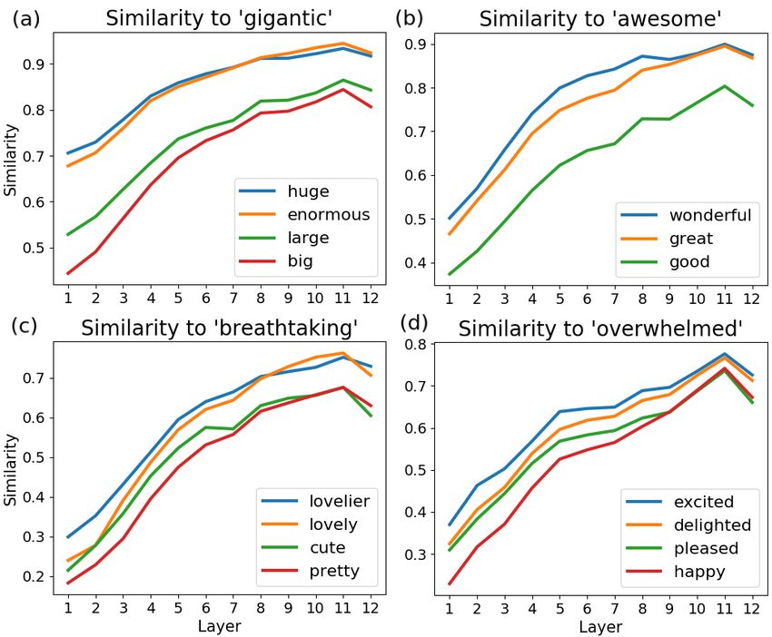
polarity as reflected in the frequency of positive vs Figure 3: Performance of DIFFVEC -1 (+) with ukWaC
negative adjectives in the two datasets. We check sentences across BERT layers.
the polarity of the adjectives in two sentiment lexi-
cons: SO-CAL (Taboada et al., 2011) and AFINN- layers, we observe that knowledge relevant for
165 (Nielsen, 2011). The two lexicons cover a scalar adjective ranking is situated in the last layers
portion of the adjectives in DE M ELO and C ROWD: of the Transformer network. Figure 3 shows how
68% and 79%, respectively. The DE M ELO dataset the performance of DIFFVEC -1 (+) changes across
is well-balanced in terms of positive and negative different BERT layers: model predictions improve
adjectives: 51% and 49% of the covered adjectives after layer 3, and performance peaks in one of the
fall in each category. In C ROWD, we observe a last four layers. This is in accordance with the
slight skew towards positive: 61% vs 39%. Accord- findings of Tenney et al. (2019) that semantic infor-
ing to this analysis, the difference in performance mation is mainly located in the upper layers of the
between the two methods could only partially be model, but is more spread across the network than
explained by an imbalance in terms of polarity. syntactic information which is contained in a few
We perform an additional analysis based on the middle layers.
Google Ngram frequency of the positive and neg-
ative words that were used for deriving DIFFVEC. 8 Conclusion
The adjectives good (276M) and awesome (10M)
We have shown that BERT representations encode
are more frequent than bad (65M) and horrible
rich information about the intensity of scalar adjec-
(4M). In fact, we find that the 1,000 most fre-
tives which can be efficiently used for their ranking.
quent positive words in SO-CAL and AFINN are,
Although our method is simple and resource-light,
on average, much more frequent (18M) than the
solely relying on an intensity vector which can be
1,000 most frequent negative words (8M). Word
derived from as few as a single example, it clearly
frequency has a direct impact on word represen-
outperforms previous work on the scalar adjective
tations, since having access to sparse information
ranking and Indirect Question Answering tasks.
about a word’s usages does not allow the model to
Our performance analysis across BERT layers high-
acquire rich information about its linguistic prop-
lights that the lexical semantic knowledge needed
erties as in the case of frequent words. The high
for these tasks is mostly located in the higher layers
frequency of good and awesome results in better
of the BERT model.
quality representations than the ones obtained for
In future work, we plan to extend our methodol-
their antonyms, and could explain to some extent
ogy to new languages, and experiment with mul-
the improved performance of DIFFVEC-1 (+) com-
tilingual and language specific BERT models. To
pared to DIFFVEC-1 (−) with BERT embeddings.
create scalar adjective resources in new languages,
However, this analysis does not explain the differ-
we could either translate the English datasets or
ence in the performance of DIFFVEC (+) and (−)
mine adjective scales from starred product reviews
between BERT and word2vec. This would require
as in de Marneffe et al. (2010). Our intention is
a better understanding of how words with differ-
also to address adjective ranking in full scales (in-
ent polarity (antonyms) are represented in BERT’s
stead of half-scales) and evaluate the capability of
space compared to word2vec, and how negation
contextualised representations to detect polarity.
affects their representations. We leave these explo-
rations for future work.
Regarding the performance of different BERT
7379Acknowledgements Christiane Fellbaum, editor. 1998. WordNet: An Elec-
tronic Lexical Database. Language, Speech, and
This work has been supported by the Communication. MIT Press, Cambridge, MA.
French National Research Agency un-
Juri Ganitkevitch, Benjamin Van Durme, and Chris
der project ANR-16-CE33-0013. The Callison-Burch. 2013. PPDB: The Paraphrase
work is also part of the FoTran project, Database. In Proceedings of the 2013 Conference of
funded by the European Research Coun- the North American Chapter of the Association for
cil (ERC) under the European Union’s Horizon Computational Linguistics: Human Language Tech-
nologies, pages 758–764, Atlanta, Georgia. Associa-
2020 research and innovation programme (grant tion for Computational Linguistics.
agreement № 771113). We thank the reviewers
for their thoughtful comments and valuable sugges- Bart Geurts. 2010. Quantity implicatures. Cambridge
University Press.
tions.
Derek Gross and Katherine J Miller. 1990. Adjectives
in WordNet. International Journal of lexicography,
References 3(4):265–277.
Marco Baroni, Silvia Bernardini, Adriano Ferraresi, Vasileios Hatzivassiloglou and Kathleen R. McKeown.
and Eros Zanchetta. 2009. The WaCky wide web: a 1993. Towards the Automatic Identification of Ad-
collection of very large linguistically processed web- jectival Scales: Clustering Adjectives According to
crawled corpora. Journal of Language Resources Meaning. In 31st Annual Meeting of the Associa-
and Evaluation, 43(3):209–226. tion for Computational Linguistics, pages 172–182,
Columbus, Ohio, USA. Association for Computa-
Tolga Bolukbasi, Kai-Wei Chang, James Y Zou, tional Linguistics.
Venkatesh Saligrama, and Adam T Kalai. 2016.
Man is to Computer Programmer as Woman is to Marti A. Hearst. 1992. Automatic Acquisition of Hy-
Homemaker? Debiasing Word Embeddings. In Ad- ponyms from Large Text Corpora. In COLING 1992
vances in Neural Information Processing Systems Volume 2: The 15th International Conference on
29, pages 4349–4357. Barcelona, Spain. Computational Linguistics.
John Hewitt and Percy Liang. 2019. Designing and
Thorsten Brants and Alex Franz. 2006. Web 1T 5-gram
Interpreting Probes with Control Tasks. In Proceed-
Version 1. In LDC2006T13, Philadelphia, Pennsyl-
ings of the 2019 Conference on Empirical Methods
vania. Linguistic Data Consortium.
in Natural Language Processing and the 9th Inter-
Kevin Clark, Urvashi Khandelwal, Omer Levy, and national Joint Conference on Natural Language Pro-
Christopher D. Manning. 2019. What does BERT cessing (EMNLP-IJCNLP), pages 2733–2743, Hong
look at? an analysis of BERT’s attention. In Pro- Kong, China. Association for Computational Lin-
ceedings of the 2019 ACL Workshop BlackboxNLP: guistics.
Analyzing and Interpreting Neural Networks for John Hewitt and Christopher D. Manning. 2019. A
NLP, pages 276–286, Florence, Italy. Association Structural Probe for Finding Syntax in Word Repre-
for Computational Linguistics. sentations. In Proceedings of the 2019 Conference
Anne Cocos, Skyler Wharton, Ellie Pavlick, Marianna of the North American Chapter of the Association
Apidianaki, and Chris Callison-Burch. 2018. Learn- for Computational Linguistics: Human Language
ing Scalar Adjective Intensity from Paraphrases. Technologies, Volume 1 (Long and Short Papers),
In Proceedings of the 2018 Conference on Em- pages 4129–4138, Minneapolis, Minnesota. Associ-
pirical Methods in Natural Language Processing, ation for Computational Linguistics.
pages 1752–1762, Brussels, Belgium. Association Christopher Kennedy and Louise McNally. 2005.
for Computational Linguistics. Scale Structure and the Semantic Typology of Grad-
able Predicates. Language, 81:345–381.
Sunipa Dev and Jeff M Phillips. 2019. Attenuating
Bias in Word Vectors. In Proceedings of the 22nd In- Adam Kilgarriff. 2004. How Dominant Is the Com-
ternational Conference on Artificial Intelligence and monest Sense of a Word? Lecture Notes in Com-
Statistics (AISTATS), Naha, Okinawa, Japan. puter Science (vol. 3206), Text, Speech and Dia-
logue, Sojka Petr, Kopeček Ivan, Pala Karel (eds.),
Jacob Devlin, Ming-Wei Chang, Kenton Lee, and pages 103–112. Springer, Berlin, Heidelberg.
Kristina Toutanova. 2019. BERT: Pre-training of
Deep Bidirectional Transformers for Language Un- Joo-Kyung Kim and Marie-Catherine de Marneffe.
derstanding. In Proceedings of the 2019 Conference 2013. Deriving Adjectival Scales from Continu-
of the North American Chapter of the Association ous Space Word Representations. In Proceedings of
for Computational Linguistics: Human Language the 2013 Conference on Empirical Methods in Natu-
Technologies, Volume 1 (Long and Short Papers), ral Language Processing, pages 1625–1630, Seattle,
pages 4171–4186, Minneapolis, Minnesota. Associ- Washington, USA. Association for Computational
ation for Computational Linguistics. Linguistics.
7380Olga Kovaleva, Alexey Romanov, Anna Rogers, and Tomas Mikolov, Kai Chen, Greg Corrado, and
Anna Rumshisky. 2019. Revealing the Dark Secrets Jeffrey Dean. 2013. Efficient Estimation of
of BERT. In Proceedings of the 2019 Conference on Word Representations in Vector Space. arXiv
Empirical Methods in Natural Language Processing preprint:1301.3781v3.
and the 9th International Joint Conference on Natu-
ral Language Processing (EMNLP-IJCNLP), pages Finn Årup Nielsen. 2011. A new ANEW: Evaluation of
4365–4374, Hong Kong, China. Association for a word list for sentiment analysis in microblogs. In
Computational Linguistics. Proceedings of the ESWC 2011 Workshop on ’Mak-
ing Sense of Microposts: Big things come in small
Gerhard Kremer, Katrin Erk, Sebastian Padó, and Ste- packages’, volume 718 in CEUR Workshop Pro-
fan Thater. 2014. What Substitutes Tell Us - Anal- ceedings, pages 93–98.
ysis of an “All-Words” Lexical Substitution Corpus.
In Proceedings of the 14th Conference of the Euro- Bo Pang, Lillian Lee, et al. 2008. Opinion mining and
pean Chapter of the Association for Computational sentiment analysis. Foundations and Trends in Infor-
Linguistics, pages 540–549, Gothenburg, Sweden. mation Retrieval, 2(1–2):1–135.
Association for Computational Linguistics.
Ajay Patel, Alexander Sands, Chris Callison-Burch,
and Marianna Apidianaki. 2018. Magnitude: A
Anne Lauscher, Goran Glavaš, Simone Paolo Ponzetto, Fast, Efficient Universal Vector Embedding Utility
and Ivan Vulić. 2020. A General Framework for Im- Package. In Proceedings of the 2018 Conference
plicit and Explicit Debiasing of Distributional Word on Empirical Methods in Natural Language Process-
Vector Spaces. In Proceedings of the 34th AAAI ing: System Demonstrations, pages 120–126, Brus-
Conference on Artificial Intelligence, New York City, sels, Belgium. Association for Computational Lin-
NY, USA. guistics.
Tal Linzen, Emmanuel Dupoux, and Yoav Goldberg. Ellie Pavlick, Pushpendre Rastogi, Juri Ganitkevitch,
2016. Assessing the Ability of LSTMs to Learn Benjamin Van Durme, and Chris Callison-Burch.
Syntax-Sensitive Dependencies. Transactions of the 2015. PPDB 2.0: Better paraphrase ranking, fine-
Association for Computational Linguistics, 4:521– grained entailment relations, word embeddings, and
535. style classification. In Proceedings of the 53rd An-
nual Meeting of the Association for Computational
Marie-Catherine de Marneffe, Christopher D. Manning, Linguistics and the 7th International Joint Confer-
and Christopher Potts. 2010. “Was It Good? It Was ence on Natural Language Processing (Volume 2:
Provocative.” Learning the Meaning of Scalar Ad- Short Papers), pages 425–430, Beijing, China. As-
jectives”. In Proceedings of the 48th Annual Meet- sociation for Computational Linguistics.
ing of the Association for Computational Linguistics,
pages 167–176, Uppsala, Sweden. Association for Peng Qi, Yuhao Zhang, Yuhui Zhang, Jason Bolton,
Computational Linguistics. and Christopher D Manning. 2020. Stanza:
A Python Natural Language Processing Toolkit
Diana McCarthy, Rob Koeling, Julie Weeds, and John for Many Human Languages. arXiv preprint
Carroll. 2004. Finding Predominant Word Senses arXiv:2003.07082.
in Untagged Text. In Proceedings of the 42nd An-
nual Meeting of the Association for Computational Shauli Ravfogel, Yanai Elazar, Hila Gonen, Michael
Linguistics (ACL-04), pages 279–286, Barcelona, Twiton, and Yoav Goldberg. 2020. Null It Out:
Spain. Guarding Protected Attributes by Iterative Nullspace
Projection. arXiv preprint arXiv:2004.07667.
Louise McNally. 2016. Scalar alternatives and scalar
Sven Rill, J. vom Scheidt, Johannes Drescher, Oliver
inference involving adjectives: A comment on van
Schütz, Dirk Reinel, and Florian Wogenstein. 2012.
Tiel, et al. 2016. In Ruth Kramer Jason Ostrove and
A generic approach to generate opinion lists of
Joseph Sabbagh, editors, Asking the Right Questions:
phrases for opinion mining applications. In Proceed-
Essays in Honor of Sandra Chung, pages 17–28.
ings of the First International Workshop on Issues
of Sentiment Discovery and Opinion Mining (WIS-
Oren Melamud, Jacob Goldberger, and Ido Dagan. DOM), pages 1–8, Beijing, China.
2016. context2vec: Learning Generic Context Em-
bedding with Bidirectional LSTM. In Proceedings Anna Rogers, Olga Kovaleva, and Anna Rumshisky.
of The 20th SIGNLL Conference on Computational 2020. A Primer in BERTology: What
Natural Language Learning, pages 51–61, Berlin, we know about how BERT works. arXiv
Germany. Association for Computational Linguis- preprint:2002.12327v1.
tics.
Josef Ruppenhofer, Michael Wiegand, and Jasper Bran-
Gerard de Melo and Mohit Bansal. 2013. Good, Great, des. 2014. Comparing methods for deriving inten-
Excellent: Global Inference of Semantic Intensities. sity scores for adjectives. In Proceedings of the 14th
Transactions of the Association for Computational Conference of the European Chapter of the Associa-
Linguistics, 1:279–290. tion for Computational Linguistics, volume 2: Short
7381Papers, pages 117–122, Gothenburg, Sweden. Asso- 57th Annual Meeting of the Association for Com-
ciation for Computational Linguistics. putational Linguistics, pages 5797–5808, Florence,
Italy. Association for Computational Linguistics.
Raksha Sharma, Mohit Gupta, Astha Agarwal, and
Pushpak Bhattacharyya. 2015. Adjective Intensity Bryan Wilkinson. 2017. Identifying and Ordering
and Sentiment Analysis. In Proceedings of the 2015 Scalar Adjectives Using Lexical Substitution. Ph.D.
Conference on Empirical Methods for Natural Lan- thesis, University of Maryland, Baltimore County.
guage Processing, pages 2520–2526, Lisbon, Portu-
gal. Association for Computational Linguistics. Bryan Wilkinson and Tim Oates. 2016. A Gold Stan-
dard for Scalar Adjectives. In Proceedings of the
Vera Sheinman, Christiane Fellbaum, Isaac Julien, Pe- Tenth International Conference on Language Re-
ter Schulam, and Takenobu Tokunaga. 2013. Large, sources and Evaluation (LREC’16), pages 2669–
huge or gigantic? Identifying and encoding intensity 2675, Portorož, Slovenia. European Language Re-
relations among adjectives in WordNet. Language sources Association (ELRA).
resources and evaluation, 47(3):797–816.
Yonghui Wu, Mike Schuster, Zhifeng Chen, Quoc V.
Vera Sheinman and Takenobu Tokunaga. 2009. AdjS- Le, Mohammad Norouzi, Wolfgang Macherey,
cales: Visualizing Differences between Adjectives Maxim Krikun, Yuan Cao, Qin Gao, Klaus
for Language Learners. IEICE Transactions on In- Macherey, Jeff Klingner, Apurva Shah, Melvin John-
formation and Systems, 92-D:1542–1550. son, Xiaobing Liu, Łukasz Kaiser, Stephan Gouws,
Yoshikiyo Kato, Taku Kudo, Hideto Kazawa, Keith
Chaitanya Shivade, Marie-Catherine de Marneffe, Eric Stevens, George Kurian, Nishant Patil, Wei Wang,
Fosler-Lussier, and Albert M. Lai. 2015. Corpus- Cliff Young, Jason Smith, Jason Riesa, Alex Rud-
based discovery of semantic intensity scales. In Pro- nick, Oriol Vinyals, Greg Corrado, Macduff Hughes,
ceedings of the 2015 Conference of the North Amer- and Jeffrey Dean. 2016. Google’s Neural Ma-
ican Chapter of the Association for Computational chine Translation System: Bridging the Gap be-
Linguistics: Human Language Technologies, pages tween Human and Machine Translation. arXiv
483–493, Denver, Colorado. Association for Compu- preprint:1609.08144.
tational Linguistics.
Peter Young, Alice Lai, Micah Hodosh, and Julia Hock-
Maite Taboada, Julian Brooke, Milan Tofiloski, Kim- enmaier. 2014. From image descriptions to visual
berly Voll, and Manfred Stede. 2011. Lexicon-based denotations: New similarity metrics for semantic in-
methods for sentiment analysis. Computational lin- ference over event descriptions. Transactions of the
guistics, 37(2):267–307. Association for Computational Linguistics, 2:67–78.
Alon Talmor, Yanai Elazar, Yoav Goldberg, and Jieyu Zhao, Yichao Zhou, Zeyu Li, Wei Wang, and Kai-
Jonathan Berant. 2019. oLMpics – On what Lan- Wei Chang. 2018. Learning gender-neutral word
guage Model Pre-training Captures. arXiv preprint embeddings. In Proceedings of the 2018 Conference
arXiv:1912.13283v1. on Empirical Methods in Natural Language Process-
ing, pages 4847–4853, Brussels, Belgium. Associa-
Ian Tenney, Dipanjan Das, and Ellie Pavlick. 2019. tion for Computational Linguistics.
BERT Rediscovers the Classical NLP Pipeline. In
Proceedings of the 57th Annual Meeting of the Asso- George Kingsley Zipf. 1945. The meaning-frequency
ciation for Computational Linguistics, pages 4593– relationship of words. Journal of General Psychol-
4601, Florence, Italy. Association for Computational ogy, 33(2):251–256.
Linguistics.
A Hearst Patterns
Bob Van Tiel, Emiel Van Miltenburg, Natalia Ze-
vakhina, and Bart Geurts. 2016. Scalar Diversity. Figure 4 illustrates the dependency structure of the
Journal of semantics, 33(1):137–175. following Hearst patterns:
Elena Voita, Rico Sennrich, and Ivan Titov. 2019a.
• [NP] and other [NP]
The Bottom-up Evolution of Representations in the
Transformer: A Study with Machine Translation and
Language Modeling Objectives. In Proceedings of • [NP] or other [NP]
the 2019 Conference on Empirical Methods in Nat-
ural Language Processing and the 9th International • [NP] such as [NP]
Joint Conference on Natural Language Processing
(EMNLP-IJCNLP), pages 4396–4406, Hong Kong, • Such [NP] as [NP]
China. Association for Computational Linguistics.
• [NP], including [NP]
Elena Voita, David Talbot, Fedor Moiseev, Rico Sen-
nrich, and Ivan Titov. 2019b. Analyzing multi-head • [NP], especially [NP]
self-attention: Specialized heads do the heavy lift-
ing, the rest can be pruned. In Proceedings of the • [NP] like [NP]
7382use data from the Concepts in Context (CoInCo)
corpus (Kremer et al., 2014). CoInCo contains sen-
tences where content words have been manually
annotated with substitutes which come with a fre-
quency score indicating the number of annotators
who proposed each substitute. We collect instances
of adjectives, nouns and verbs in their base form.18
For a word w, we form instance pairs (wi -wj with
i 6= j) with similar meaning as reflected in their
shared substitutes. We allow for up to two unique
substitutes per instance, which we assign to the
other instance in the pair with zero frequency. We
keep instances with n substitutes, where 2 ≤ n ≤
8 (the lowest and highest number of adjectives in a
scale). This results in 5,954 pairs.
We measure the variation in an instance pair in
terms of substitutes using the coefficient of varia-
tion (VAR). VAR is the ratio of the standard devi-
ation to the mean and is, therefore, independent
from the unit used. A higher VAR indicates that not
all substitutes are good choices in a context. We
keep the 500 pairs with the highest VAR difference,
where one sentence is a better fit for all substitutes
than the other. For example, private, individual and
person were proposed as substitutes for personal
in “personal insurance lines”, but private was the
preferred choice for “personal reasons”. The tested
methods must identify which sentence in a pair is
a better fit for all substitutes.
For sentence selection, we experiment with the
three fluency calculation methods presented in
Section 4.2: BERT PROB (the BERT probability
of each substitute to be used in the place of the
[MASK] token); BERT PPX (the perplexity as-
signed by BERT to the sentence generated through
substitution); and CONTEXT 2 VEC (the cosine simi-
Figure 4: Dependency structure of Hearst patterns. larity between the context2vec representations of a
substitute and the context).
We also test VAR and standard deviation (STD)
We use these patterns to detect sentences where
as metrics for measuring variation in the fluency
adjective substitution should not take place, as
scores assigned to a sentence pair by the three meth-
described in Section 4.2 of the paper. We re-
ods. We evaluate the sentence selection methods
move these sentences from our ukWaC and Flickr
and variation metrics on the 500 pairs retained from
datasets.17
CoInCo. We report their accuracy, calculated as
B Evaluation of Sentence Selection the proportion of pairs where a method correctly
Methods guesses the instance in a pair with the lowest varia-
tion. We compare results to those of a baseline that
To identify the most appropriate method for select- always proposes the first instance in a pair. The
ing sentences where all adjectives in a scale fit, we results in Table 6 show that the task is difficult for
17 18
Graphs in Figure 4 were created with the visualisation tool This filtering serves to control for morphological variation
available at https://urd2.let.rug.nl/˜kleiweg/ which could result in unnatural substitutions since CoInCo
conllu/ substitutes are in lemma form.
7383You can also read