Causal reductionism and causal structures - Center for Sleep and ...

Causal reductionism and causal structures
 Matteo Grasso, Larissa Albantakis, Jonathan P. Lang, Giulio Tononi
 Department of Psychiatry, University of Wisconsin-Madison

 Appendix
Appendix A: Environment and task

 In this study we use the formal framework of actual causation (Albantakis et al., 2019) to provide a causal analysis of three
kinds of artificial organisms (‘frogs’) created in silico and exposed to a simulated environment. All frogs were modeled to
live in a two-dimensional grid world containing three kinds of other organisms (‘bugs’) (see Fig. 1). Left-bugs and right-
bugs (‘small-bugs’) occupy two horizontally adjacent squares and are composed of a head (black square) and a tail (white
square). They preferentially move in the direction of their head (left for left-bugs, right for right-bugs) and occasionally move
in the three remaining cardinal directions. Left- and right-bugs are prey and do not react to their surroundings. Super-bugs
occupy three horizontally adjacent squares and have two heads at their extremities (black squares) and a body in the middle
(white square). They preferentially move straight down but can also move diagonally downward if they detect an object
below them. Super-bugs are predators and prey on frogs and all other kinds of bugs.
 F3 and F2 frogs occupy a surface of 3x3 squares. They stay still if they do not detect any object, they move diagonally
upward (‘jump left’ or ‘jump right’ action) if they detect a black square with the respective eye, and move up three squares
(‘jump over’ action) if they detect black squares with both their eyes. F3 and F2 frogs prey on small-bugs (‘caught’ scenario,
when overlapping with a small-bug) and are preyed on by super-bugs (‘Dead!’ scenario, when overlapping with a super-
bug).
 F1 frogs occupy three vertically adjacent squares and remain still if they do not detect any object. They can be of two kinds,
left-half-frogs or right-half-frogs, and preferably move diagonally up-left or up-right, respectively, when they detect a black
square above them and a white square to the left or right, respectively. Left-half frogs are thus specialized to detect and catch
left-bugs, while right-have frogs are specialized to detect and catch right-bugs. Like F3 and F2 frogs, F1 frogs prey on small-
bugs and are preyed on by super-bugs (Fig. A1).

 Figure A1: Environment and behavior of F1 frogs.

 1

Appendix B: Causal analysis

 All frogs are constituted by three kinds of probabilistic binary units: sensors (S), central units (C), and motors (M) (Fig.
2). The probability p of a given unit to fire is defined according to the following activation function:
 2
 1 ( , , ) − 
 − ( )
 2 
 ( , +1 → ) = 

where i is the index of the current unit, j is an index over its inputs, s = {0,1} denotes the binary state of the (ith or jth) unit
at time t (for the current state) or t+1 (for the output state), w is the connection weight between the ith and jth unit (see
connection weights in Fig. B1, panels A-C),  = 1 and  = 0.3 (Fig. B1, panel D). For example, in F2 frogs, the sum of unit
ML’s input connection weights equals 1 when the state of its inputs is CLCR = 11, and the probability that unit ML will fire
equals 1.
 The dynamics of each system (its global update function) can be fully described by a state transition probability matrix
(TPM) which specifies the probability of any system to transition between any two states. Based on the frogs’ TPMs, we
have conducted a causal analysis to determine which subsets of central units form irreducible mechanisms in each case and
to identify the actual cause and effect of each mechanism in its state at time t. Here, we have focused our causal analysis on
mechanisms constituted by central units, since only central units have both causes and effects within the frogs’ nervous
system.
 For a particular subset of central units in its state at time t, we apply the principle of integration to determine how much
irreducible cause information it specifies about all possible sets of sensor units (cause purviews) at t-1. Likewise, we measure
how much irreducible effect information it specifies about all possible sets of motor units (effect purviews) at t+1. The
irreducible information is computed according to the actual causation framework (Albantakis et al., 2019) in terms of the
causal strength (). In simplified terms, for a mechanism Y in state and a cause purview in state −1, cause is defined
as:
 ( −1 | )
 cause = ( −1| ) 2 ( ),
 ( ( −1| ))

and effect over the effect purview in state +1 as:
 ( +1 | )
 effect = ( +1 | ) 2 ( ).
 ( ( +1 | ))

 Above, ( ±1 | ) is the probability of the purview state for the unpartitioned mechanism, and Ψ ( ( ±1 | )) is the
probability of the purview state after partitioning the mechanism into ( 1, ±1 | 1, ) × ( 2, ±1 | 2, ). Note that here
does not simply correspond to observed probabilities, but to the interventional probabilities obtained from the system’s TPM

 Figure B1: Connection weights and unit activation function.

 2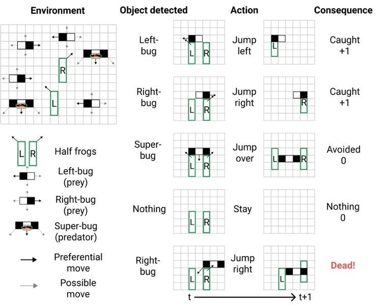

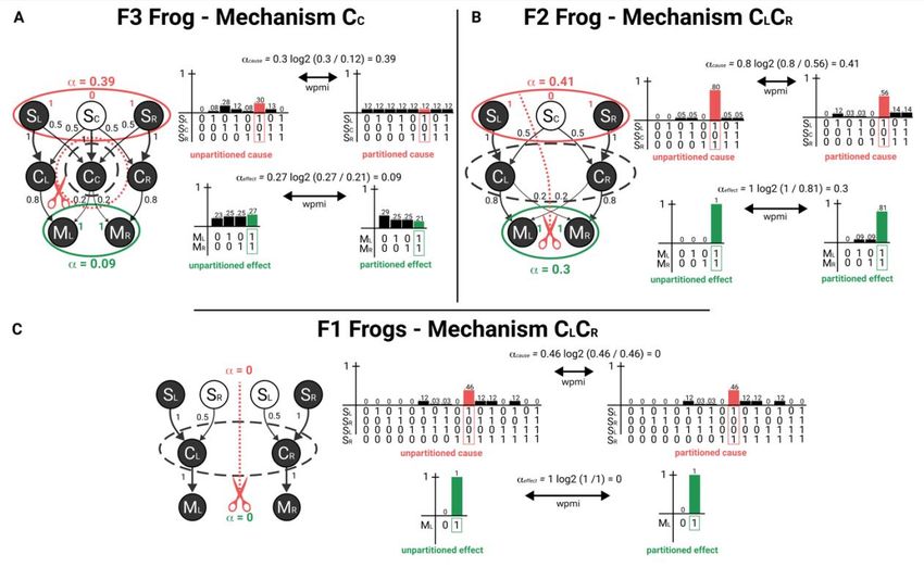
and is technically a product distribution to discount non-causal correlations between units (see Albantakis et al. (2019) for
details).
 Moreover, in line with (Barbosa et al., 2020),  here is formalized as a measure of Intrinsic Difference, an information
measure that balances expansion and dilution. As such, the log ratio between the probability of the purview state before (p)
 
and after (q) the mechanism is partitioned is weighted by p, resulting in an equation of the form = ∗ log 2 . Adding this
weighing factor provides a tradeoff between increased purview size and increased noise, which prevents including units in
the cause or effect that only contribute a miniscule amount, especially in the presence of noise in the system.
 Among all irreducible cause purviews, the cause purview with the highest value of  is selected as the actual cause. This
corresponds to applying the exclusion principle, according to which the actual cause of a mechanisms is the cause about
which the mechanism specifies the most irreducible information and therefore upon which the mechanism exerts maximal
causal strength (the exclusion principle is applied, mutatis mutandis, to select the actual effect).
 In the main text, we explicitly discuss the results of causal analysis for three mechanisms: C C in F3 frogs, and CLCR in F2
and pairs of F1 frogs. The system state in each case corresponds to the scenario where a super-bug is encountered, which
leads to the firing of all central units and a subsequent escape action. Details of causal analysis for these mechanisms are
shown in Fig. B2.
 For instance, in F3 mechanism CC specifies a conditional probability distribution by being in state CC = 1 at t over the
possible states of the input units SLSCSR at time t-1, CC’s cause purview (Fig. B2, panel A, unpartitioned cause).
 The minimal partition is indicated by the red dotted line around mechanism C C, which in this case replaces all input
connections to mechanism CC with noise. The effect of the partition is shown, again, as a probability distribution over all
states of the mechanism’s input units (Fig. B2, panel A, partitioned cause).
 The irreducibility of CC = 1 over the cause purview is then assessed by its cause value, inserting the probability of the
purview’s actual state SLSCSR = 101, before and after partitioning the mechanism in the equation above.
 This procedure is performed for all possible cause purviews (subset of SLSCSR, such as SLSC or SCSR). SLSCSR = 101 is
selected as the actual cause of the CC = 1, since it is the one that yields the highest value of  (the comparison with other
irreducible purviews is omitted).
 Similarly, causal analysis of the second-order mechanism CLCR in F2 shows that this mechanism also specifies an
irreducible cause purview, over units SLSCSR = 101 at t-1, because the probability of its cause purview SLSCSR = 101 at t -1
given that CLCR = 11 at t is reduced by partitioning the mechanism (in Fig. B2 panel B the red dashed line indicates that the
connection from unit SC to mechanism CLCR is noised). Also in this case SLSCSR = 101 yields the highest value of .
 By contrast, causal analysis of the second-order mechanism CLCR in the pair of F1 frogs shows that this mechanism does

 Figure B2: Causal analysis of selected mechanisms.

 3

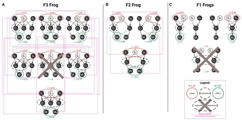
Figure B3: Causal structure of F3, F2 and pairs of F1 frogs.
not specify an irreducible cause purview over the input units SLSRSLSR = 1001 (or any subset) at t-1, because there is at least
one way to partition the mechanism that makes no difference to the probability SLSRSLSR being in state 101 at t-1 given that
CLCR = 11 at t. Thus, the current state of mechanism C LCR does not specify irreducible information about the state of its
inputs SLSRSLSR at t-1 (Fig. B2, panel C).
 The full causal structure of each frog is presented in Fig. B3. F3 frogs specify 6 irreducible mechanisms with specific
causes and effects, and with many causal relations that arise when purviews overlap on the units they irreducibly constrain
(indicated by purple edges in Fig. B3) (Haun & Tononi. 2019). In addition to mechanism CC = 1 with its actual cause SLSCSR
= 101 (which corresponds to detecting a super-bug) and its actual effect MLMR = 11 (which corresponds to jumping over),
the causal structure of F3 includes two more first-order mechanisms, CL = 1 and CR = 1, with their actual cause SLSC = 10
(which corresponds to detecting a left-bug) and units SCSR = 01 (which corresponds to detecting a right-bug), respectively
(and likewise their respective effects).
 CL = 1 and CR = 1 are causally related, as their actual causes overlap over unit S C = 0, reflecting something that left- and
right-bugs have in common – a tail in the middle of the frog’s visual field (see purple edge connecting the cause purviews of
the two mechanisms in Fig. B3, panel A). A further fact visible in the causal structure of F3 frogs is that the actual cause
SLSCSR = 101 of CC = 1 is equivalent to the union of the actual causes of CL = 1 and CR = 1:
 ( = 101) = ( = 10) ∪ ( = 01).
 This also reflects a fact about the world, namely, that superbugs are composed of a left-bug and a right-bug fused by the tail.
Similar considerations can be made for the effect side and the relations between the actions of jumping left, jumping right,
and jumping over.
 Contrary to the reductionist account of F3 frogs, the full causal analysis actually reveals that some higher-order mechanisms
also exist in F3 frogs. The causes and effects of these higher-order mechanisms are congruent with the causes and effects of
the first-order mechanisms and thus give rise to additional causal relations, but also reveal further differences between the
three types of frogs.
In F2 frogs, all of the 3 possible mechanisms (CL, CR, and CLCR, 2 first-order and 1 second-order) are irreducible, with
specific causes and effects, and the causal relations between their actual causes and effects again reflect the relations between
the objects in the environment and the actions performed by F2 frogs.
 Analyzing the pair of F1 frogs, it can easily be shown that their joint causal structure is reducible into two separate causal
structures, one for each frog, with one first-order mechanism each. Accordingly, there is no second-order mechanism that
spans the central units of the two frogs: the subset C LCR is reducible (Fig. B2, panel C).As a consequence, no relation can
be found between actual causes and effects of mechanisms C L and CR, showing that not only do pairs of F1 frogs not detect
superbugs, but also that the relations between objects in the world and actions performed is nowhere to be found in the causal
structure they specify alone or together (Fig. B3, panel C).

 4

Appendix C: Macro and micro causation example

 System description: At the micro level the example system is constituted of nine interacting elements, arranged into three
functional units A, B, and C (also referred to as “macro units” or “black boxes”). Each functional unit has two micro input
units X and Y, which have two states each ({0,1}), and one micro output unit O that can take three different states ({0,1,2}).
All X and Y receive input from all three output units OA, OB, and OC (short OABC). The inputs from other functional units are
excitatory, while the input from the same functional unit is inhibitory (e.g., OA recurrently inhibits XA and YA). Each output
O receives excitatory inputs from X and Y within the same functional unit.
 The activation function of all X and Y units corresponds to a sigmoid function that determines the probability of a unit X
or Y to be in state 1 given the previous state of its inputs { , −1 , , −1 , , −1 }. As an example, the activation function for
unit XA is as follows:

 −1
 2(− , −1 + , −1 + , −1 +ℎ)
 −
 ( , = 1| , −1 ) = (1 + )

with a bias ℎ = −1.8 that decreases the probability of firing (X = 1), and some amount of indeterminism = 0.4. The same
parameters were used for all X and Y units.
 The activation function of all ternary output units O corresponds to a softmax function over its inputs X and Y:

 ( = | −1 ) =
 ∑ 

with , ∈ {0,1,2} and = [[3.5, 2.5, 2.0], [2.0, 3.0, 3.0], [1.0, 2.0, 5.0]]. Thus, if the inputs to O sum to 2, for example, the
probabilities of O being in state 0, 1, or 2 are determined by [1.0, 2.0, 5.0], which means that the most likely state of O is 2.
From these equations, all transition probabilities at the micro and macro levels can be calculated, which form the basis of the
causal analysis presented in Box 2 of the main paper (see details below).

 Causal analysis: As a proof of principle that the causal strength of macro causes and effects may exceed that of their
underlying micro causes and effects, we compared the causal strength of the cause of output unit (or its corresponding
functional unit ) under various macro grains of description (see Figure B.3, main text) for the maximally activated state of
 
the system. As in the main example, causal strength was calculated as = ∗ log according to (Albantakis et al., 2019)
paired with (Barbosa et al., 2020), where denotes the probability of the state of the inputs of (or ) to be in their
maximally activated state given the state of (or the black box ) and q corresponds to the same probability but under a
full partition of the connections between (or ) and its inputs. At the macro grain size of the functional units, A, B, and
C are evaluated as black boxes as described in Marshall et al. (2018), which function over two micro time steps and whose
state is determined by the state of their respective output element O.

References
 Albantakis, L., Marshall, W., Hoel, E., & Tononi, G. (2019). What caused what? A quantitative account of actual causation using dynamical causal
networks. Entropy, 21(5), 459.
 Barbosa L.S., Marshall, W., Streipert, S., Albantakis, L., Tononi, G. (2020). A measure for intrinsic information. Sci Rep 10:18803.
 Haun, A., & Tononi, G. (2019). Why does space feel the way it does? Towards a principled account of spatial experience. Entropy, 21(12), 1160.
 Marshall, W., Albantakis, L., & Tononi, G. (2018). Black-boxing and cause-effect power. PLoS computational biology, 14(4), e1006114.

 5