CEP Discussion Paper No 1681 March 2020 On the Economic Impacts of Mortgage Credit Expansion Policies: Evidence from Help to Buy Felipe Carozzi ...

ISSN 2042-2695

 CEP Discussion Paper No 1681
 March 2020

On the Economic Impacts of Mortgage Credit Expansion
 Policies: Evidence from Help to Buy

 Felipe Carozzi
 Christian Hilber
 Xiaolun Yu

Abstract
Mortgage credit expansion policies – such as UK’s Help to Buy (HtB) – aim to increase access to and
affordability of owner-occupied housing and are widespread around the world. We take advantage of spatial
discontinuities in the HtB equity loan scheme, introduced in 2013, to explore the causal economic impacts and
the effectiveness of this type of policies. Employing a Difference-in-Discontinuities design, we find that HtB
increased house prices by more than the expected present value of the implied interest rate subsidy and had no
discernible effect on construction volumes in the Greater London Authority (GLA), where housing supply is
subject to severe long-run constraints and housing is already extremely unaffordable. HtB did increase
construction numbers without affecting prices near the English/Welsh border, an area with less binding supply
constraints and comparably affordable housing. HtB also led to bunching of newly built units below the price
threshold, building of smaller new units and an improvement in the financial performance of developers. We
conclude that credit expansion policies such as HtB may be ineffective in tightly supply constrained and already
unaffordable areas.

Key words: help to buy, house prices, construction, housing supply, land use regulation
JEL Codes: G28; H24; H81; R21; R28; R31; R38

This paper was produced as part of the Centre’s Urban Programme. The Centre for Economic Performance is
financed by the Economic and Social Research Council.

We thank Paul Cheshire, Pierre-Philippe Combes, Gilles Duranton, Steve Gibbons, Ingrid Gould Ellen, Hans
Koster, Stanimira Milcheva, Henry Overman, Ruchi Singh, Mark Stephens, Jos Van Ommeren and
conference/seminar participants at the Penn-Oxford Symposium on Housing Affordability in the Advanced
Economies, the European meeting of the Urban Economics Association in Amsterdam, the ESCP Europe-TAU-
UCLA Conference on Low-Income Housing Supply and Housing Affordability in Madrid, the Ministry for
Housing, Communities and Local Government, the European Regional Science Congress in Lyon (special
session), the "Public Policies, Cities and Regions" Workshop in Lyon, the London School of Economics,
University College London and Tinbergen Institute for helpful comments and suggestions. We thank Hans
Koster and Ted Pinchbeck who provided code helping us to merge Land Registry and Energy Performance
Certificate data. Financial support from Fruition Properties (through LSE Advancement) and STICERD are
gratefully acknowledged. This is a slightly revised version of the paper that won the 2019 Nick Tyrrell Research
Prize. All errors are the sole responsibility of the authors.
We are grateful to Richard Layard for helpful comments and suggestions.
 Felipe Carozzi, London School of Economics and Centre for Economic Performance, LSE. Hilber,
London School of Economics and Centre for Economic Performance, LSE. Xialun Yu, London School of
Economics.

Published by
Centre for Economic Performance
London School of Economics and Political Science
Houghton Street
London WC2A 2AE

All rights reserved. No part of this publication may be reproduced, stored in a retrieval system or transmitted in
any form or by any means without the prior permission in writing of the publisher nor be issued to the public or
circulated in any form other than that in which it is published.

Requests for permission to reproduce any article or part of the Working Paper should be sent to the editor at the
above address.

 F. Carozzi, C. Hilber and X. Yu, submitted 2020.

1. Introduction
Government policies directed at stimulating supply or demand in mortgage markets are
common throughout the world. Examples of credit market interventions include mortgage
interest deductions in countries as diverse as the United States, India or Sweden, mortgage
guarantees in the United States or the Netherlands, and government loans for home purchases
in France or the United Kingdom. Most of these interventions have the explicit goal of making
homeownership more affordable and thus accessible. In a context in which housing
affordability problems are increasingly pervasive, especially in large desirable cities, new
policies are discussed – if not implemented – frequently. In this paper, we exploit a unique
setting – spatial discontinuities in an equity loan scheme – to shed light on the economic impacts
and the effectiveness of publicly-funded credit market expansion policies, and, in particular of
government equity loans.

In April 2013, the British government launched a new flagship housing credit policy: Help to
Buy (HtB). The program was initially implemented in England, but Welsh and Scottish versions
were put in place shortly thereafter. We set out to explore the causal impact of HtB on housing
construction, house prices, the size of newly constructed units and the financial performance of
residential developers. To do so, we focus on the HtB ‘Equity Loan Scheme’, which provides
an equity loan for up to 20% of the housing unit’s value – or 40% within the Greater London
Authority (GLA) – to buyers of new build properties. The Equity Loan Scheme is by far the
most salient and popular of the four HtB schemes and the one requiring the biggest budget. It
is often referred to simply as “Help to Buy” and henceforth, unless we note otherwise, when
we refer to HtB we mean the Equity Loan Scheme.1

HtB expands housing credit and thus increases demand for housing. To explore how such a
positive demand shock in the housing market affects construction and prices, we develop a
simple theoretical framework with heterogeneous households and credit constraints. Our model
predicts that the impact of the policy depends crucially on the responsiveness of supply to
prices. In a setting with responsive supply, HtB can be expected to mainly stimulate
construction numbers as intended by the policy. However, when supply is unresponsive (i.e.,

1
 At the time of implementation, HtB consisted of four schemes; the Equity Loan Scheme, Mortgage Guarantees,
Shared Ownership, and Individual Savings Accounts (ISA). All four schemes aim to help credit constrained
households to buy a property. The Mortgage Guarantees scheme ceased at the end of 2016. The HtB-ISA closes
for new entrants in November 2019 and any bonus must be claimed by 2030. In April 2017, the British government
introduced a new Lifetime ISA scheme. In contrast to HtB ISA, it is only open to individuals aged 18-39 and the
money saved can also be used to fund a pension.

 1

regulatory constraints or physical barriers to residential development impede a supply-
response), the effect of the policy may be mainly to increase house prices, with the unintended
consequence of making housing less rather than more affordable.

We implement a Difference-in-Discontinuity design to compare changes in house prices and
construction activities across jurisdictional boundaries. We separately analyze properties sold
on either side of the GLA boundary and on either side of the English/Welsh border. In both
cases we only consider housing purchases close to the respective boundaries. As pointed out
above, in Wales the scheme was put in place later and it only applied to a subset of the properties
that were eligible in England. Likewise, the London scheme that was implemented in 2016
offered larger government equity loans (as a share of house values) for dwellings inside the
GLA compared to those available for purchase outside the GLA. Our main estimates exploit
these spatial discontinuities to study the effect of HtB on house prices and construction activity.
We also use this design to study the impact of the scheme on the size of newly constructed
units.

We focus on the GLA boundary and the English/Welsh border for two reasons. First, our
research design requires spatial discontinuities in the scheme’s conditions, which can be found
at these boundaries. Second, the two areas differ starkly in their regulatory land use
restrictiveness and in barriers to physical development: While the GLA is the most supply
constrained and the least affordable area in the UK – and arguably one of the most supply
constrained areas in the world – housing supply is comparably responsive to demand shocks
near the English/Welsh border.2

Consistent with our theoretical predictions, we find that differences in the intensity of the HtB-
treatment have heterogeneous effects depending on local supply conditions. In the GLA, where
supply is relatively unresponsive to price changes, the introduction of the more generous
London version of the Equity Loan Scheme led to a significant increase in prices for new build
units of roughly 6%. However, it had no appreciable effect on construction activity. Conversely,
in the areas around the English/Welsh border, where only a small fraction of land is developed
and developable land is readily available, we find a significant effect on construction activity
and no effect on prices. The introduction of the more generous HtB-price threshold on the
English side of the border increased the likelihood of a new build sale by about 8% (compared
to the Welsh side of the border). Consistent with this, a bunching analysis reveals that HtB led

2
 We provide supporting evidence for this proposition in Section 3.2.

 2

to significant bunching of properties right below the price threshold, shifting construction away
from larger properties above the threshold towards smaller units. We also provide evidence
indicating that the scheme caused an improvement of the financial performance of developers;
larger revenues as well as higher gross and net profits.

Collectively, these results suggest that the effects of HtB largely depend on local supply
conditions. We find that the scheme fails to trigger more construction activity, but instead
causes house prices to increase inside the GLA, precisely the region that is most affected by the
‘affordability crisis’. This has distributional implications. The main beneficiaries of HtB in
already unaffordable areas may be developers and landowners rather than struggling first-time
buyers; while access to homeownership is improved in principle (credit constraints are relaxed),
the present value of the financial burden associated with the purchase of a home further
increases.

Our paper relates to previous studies looking at the effects of credit conditions and credit market
policies on housing markets. Previous research in this vast literature has mainly focused on the
effect of credit supply on house prices (see Stein 1995, Ortalo-Magné and Rady 2006, Mian et
al. 2009, Duca et al. 2011, Favara and Imbs 2015). These and other studies provide theoretical
and empirical credence to the notion that expansions in credit supply lead to higher prices,
especially in areas with tight planning conditions. On the policy evaluation front, several studies
have explored the impact of demand subsidies on housing market outcomes. Hilber and Turner
(2014) examine the impact of the U.S. mortgage interest deduction (MID). They find that the
MID boosts homeownership attainment only of higher income households in markets with lax
land use regulation. In tightly regulated markets with inelastic long-run supply of housing, the
MID lowers homeownership attainment, presumably because higher house prices also raise
down-payment constraints of would-be-buyers. Sommer and Sullivan (2018) estimate a
dynamic structural model of the housing market to study the effect of removing the MID and
predict this would result in a substantial reduction in house prices. Finally, a significant
literature has studied the effect of credit expansion policies in the US – such as FHFA
guarantees and GSE lending – on homeownership attainment, finding mixed results. 3 Our
analysis contributes to this literature by documenting how a credit expansion-policy affects
prices, construction activity and developer performance. We interpret our results as the

3
 See for example Bostic and Gabriel (2006), Gabriel and Rosenthal (2010) and Fetter (2013). Olsen and Zabel
(2015) review the US literature. A comparison of US policies with policies in the UK and Switzerland can be
found in Hilber and Schöni (2016). An evaluation of the French Pret a Taux Zero policy – which provides a down-
payment subsidy to low and middle-income first-time buyers can be found in Gobillon and le Blanc (2008).

 3

predictable outcome of an exogenous credit expansion shock, which helps link our estimates to
the broader literature on mortgage supply and housing markets.

Only a very limited number of studies have shed light on the effects of HtB on housing and
mortgage markets. Finlay et al. (2016) estimate that since its introduction HtB has generated
43% additional new homes. They conclude that the scheme has been successful in increasing
housing supply. While their analysis combines quantitative and qualitative methods, their study
lacks proper identification of the effects using a rigorous empirical approach. Szumilo and
Vanino (2018) use a spatial discontinuity approach similar to the one employed here but focus
their analysis on the effect of HtB on lending volumes only. Benetton et al. (2019) explore the
effect of HtB on households’ house purchase and financing decisions. Applying a Difference-
in-Difference strategy, they find that households take advantage of an increase in the HtB
maximum equity limit to buy more expensive properties. To date, we have no state-of-the-art
evaluation of the impacts of the policy on house prices and construction volumes. Our paper
aims to address this.

Finally, this paper links to previous research on housing and land supply, including work on the
effects of supply constraints on the responsiveness of housing markets to economic shocks
(Hilber and Vermeulen, 2016), the origin of supply restrictions (Saiz 2010, Hilber and Robert-
Nicoud, 2013) and their consequences (see Gyourko and Molloy 2015 and the references
therein). We contribute to this literature by studying in depth the effect on housing supply of
arguably the most important new British housing policy since the implementation of Right to
Buy in 1980.

The rest of this paper is structured as follows. Section 2 describes the details of the HtB Equity
Loan Scheme and provides a simple theoretical framework to guide the empirical analysis.
Section 3 outlines our empirical strategy and discusses the results. Section 4 concludes.

2. Background and Theoretical Framework
2.1. Background: The Help to Buy Equity Loan Scheme

Since the launch of HtB in April 2013 until September 2018, over 195,000 properties were
bought with a government equity loan provided by the scheme. The total value of these loans
is £10.7 billion, with the value of the properties purchased under the scheme totaling £49.9
billion (Ministry of Housing, Communities and Local Government 2019).4

4
 The Ministry of Housing, Communities and Local Government (2019) provides a comprehensive overview and
numerous summary statistics relating to the HtB Equity Loan Scheme.

 4

The English version of the HtB Equity Loan Scheme offers government loans of up to 20% of
a unit value to households seeking to buy a new residence. It is available to both first-time
buyers and home-movers but it is restricted to the purchase of new build units with prices under
£600,000. Given that the prevalent maximum Loan-to-Value (LTV) ratios offered by British
banks to first-time buyers were around 75% during this period, the scheme offers a substantial
reduction in the down-payment needed to buy a property. With the government loan covering
part of the down-payment, buyers are only required to raise 5% of the property value as a
deposit. The explicit goal of the Equity Loan Scheme is that this reduction in the deposit
required to the borrower helps households overcome credit constraints.

The Equity Loan Scheme can also help reduce household borrowing costs by reducing interest
payments on the combined loan. This occurs via two channels. The first is that no interest or
loan fees on the equity loan have to be paid by the borrower for the first five years after the
purchase of the house. Subsequently, there is a charge, which depends on the rate of inflation.
We calculate the implied subsidy provided through this channel in Section 3.7. Secondly, by
raising the combined deposit to 25%, the equity loan keeps borrowers away from high-LTV,
high-interest products available in the commercial mortgage market.5

The government equity loan can be repaid at any time without penalty. However, unless they
want to sell the property, borrowers do not need to repay the loan at all. When they sell, the
government will reclaim its 20% equity stake of the sale price. The government thus participates
in capital gains and losses.

In our analysis we exploit differences between the English, Welsh and London versions of the
Equity Loan Scheme. The Welsh scheme was introduced in January 2014 and provided support
for the purchase of properties with prices under £300,000.6 The London scheme was introduced
in February 2016 and offered an equity loan of up to 40% of the unit’s price for properties under
£600,000 located within the GLA. The regional differences in the scheme are summarized in
Table 1.

One important feature of the different loan schemes is that they are only available for the
purchase of newly built properties. This condition is intended to leverage the increase in

5
 This enables households to gain access to more attractive mortgage rates from lenders who participate in the
scheme. Eligibility conditions require borrowers to have a suitable credit score and to be able to cover the monthly
repayments.
6
 Scotland also introduced a HtB Equity Loan Scheme during 2014; however, we are not able to exploit the
discontinuities at the English/Scottish border. This is because the Scottish Land Registry did not identify new build
units until 2018.

 5

demand for these properties with the ultimate aim of triggering a supply response. It implies
that demand faced by residential developers, construction companies and other actors in the
construction sector will increase with the policy. We use information from these companies’
accounting data to estimate the effect of the policy on their financial performance.

2.2. Theoretical Framework

In this sub-section we develop a theoretical framework to guide our empirical analysis. 7
Specifically, we develop a simple model of the housing market with heterogeneous households,
featuring credit constraints and endogenous housing supply. It is a partial equilibrium model in
that we abstract from potential effects of changing credit conditions for new builds on the price
of the existing stock.

The framework illustrates how a relaxation of credit conditions affects housing quantities and
prices, and how these effects depend on the costs of developing new stock. A relaxation of
credit constraints leads to both an increase in prices and an expansion in quantities. Under
suitable assumptions – made explicit below – the relative magnitude of the two effects depends
on the responsiveness of supply to prices. For low (high) supply responsiveness, the price effect
is stronger (weaker) and the quantity effect weaker (stronger). The theoretical insights from this
framework can be summarized by the cross-elasticities of quantity and prices taken over the
credit conditions parameter and a building cost shifter.8 We also show how a relaxation of credit
conditions can increase developer profits.

Suppose a two-period economy with a unit mass of households with preferences over a
numeraire consumption good and housing ℎ, as given by a period utility ( , ℎ) which is
continuous, strictly increasing and differentiable in both arguments. Assume in addition that
lim ( , ℎ) = ∞ if > 0 and ( , ℎ) > 0 ∀ , ℎ > 0. Households enjoy utility at the end of
ℎ→∞

periods 1 and 2, and the discount factor is β>0.

Households can only obtain ℎ > 0 if they buy a new unit and obtain housing consumption
normalized to 0 otherwise. We can think of these alternatives either as a choice between renting
and buying. In this interpretation, this formulation is similar to those used in models featuring
warm-glow from ownership (Iacoviello and Pavan 2013, Kiyotaki et al. 2011, Carozzi 2019).

7
 The model builds on Hilber and Vermeulen (2016) who consider a similar setting but abstract from the role of
credit conditions.
8
 The model presented here introduces credit conditions via a change in required loan-to-value ratios (LTVs), as
is customary in the literature. We treat housing as homogeneous, with all built units being identical in the utility
they provide to households, but heterogeneous in development costs.

 6

The role of the assumption is to ensure that demand for new build units is determined solely by
credit conditions.

Households receive an endowment in period 1 and a location specific income in period 2
which can be used for consumption or to buy property. Households are heterogeneous in the
initial endowment , which is continuously distributed over the unit interval [0,1] with
cumulative density function . In period 2, income is .

New build units are homogeneous and can be bought in period 1 for an endogenous price P.
Credit is available for the purchase of property, yet a minimum down-payment is required
corresponding to a fraction (1 − ) of the property value. Credit and savings pay interest . We
 
assume that > (1 + ) which ensures that, for sufficiently large ℎ, demand for new build
 1− 

units is determined solely by the credit constraint.9 Hence, demand is given by the mass of
agents that can afford a down-payment = 1 − ((1 − ) ) . Note that demand is
downward sloping as the function is strictly increasing.

There is a unit mass of developable land which can be used to build – at most – a unit mass of
housing units. Development costs for new build units depend on local supply conditions and
are heterogeneous across land plots. We assume that the development costs are uniformly
distributed in the [0, ] interval, with (1 − ) > 1. We assume land is owned by competitive
firms which will develop their plot if the price is smaller than or equal to development costs.
As a result, the new build inverse supply curve for competitive developers is given by = .
High values of correspond to higher average development costs and, therefore, to a weaker
response of quantities to a change in prices. Conversely, low values of are associated with a
more responsive supply schedule (i.e. a flatter supply curve). We can substitute this expression
in demand to obtain an implicit definition for new build equilibrium quantities:

 ∗ = (1 − ((1 − ) ∗ )) (1)

By differentiating this expression, we can obtain the following four statements regarding the
responses of equilibrium prices and quantities to changes in credit conditions ( ) , and
development costs ( ):
 ∗ ∗ ∗ ∗
 0 >0 >0 (2)
 
9 1 
 Note that ≤ . Assumption > (1 + ) will therefore ensure that in period 2 all agents are able to pay
 1− 1− 
the remaining part of any loans taken for the purchase of a property, including interest. Large enough ℎ ensures
buying property in period 1 is incentive compatible for all households. See theoretical Appendix.

 7

The first two inequalities indicate that an increase in development costs results in a reduction
in equilibrium quantities and an increase in equilibrium prices. 10 The third and fourth
inequalities mean that both quantities and prices respond positively to an expansion of credit.
This follows from the increase in demand associated with a credit expansion. The extent to
which a change in credit conditions will translate into a change in quantities or prices depends
on both the distribution of the initial endowment and the price responsiveness of supply
(through ).

Proposition 1 – The effect of a credit expansion on prices and quantities depends on the
distribution of development costs, as measured by . Specifically, if is uniformly distributed
 
and (1 − ) > 1, then

reasonable in our case, as the residential construction market is characterized by substantial
concentration and high returns. We test empirically whether Proposition 2 is satisfied in Section
3.

3. Empirical Analysis
3.1. Data and Descriptive Statistics

Our empirical analysis employs geo-located data on housing sales in England and Wales,
including information on unit characteristics and transaction prices. Our main data source is the
Land Registry Price Paid Dataset (or short ‘Land Registry’), which covers most residential and
all new build residential transactions in England and Wales. The dataset includes property sales
from 1995 to 2018, recording the transaction price, postcode, address, the date the sale was
registered (which proxies for the transaction date), and categorical data on dwelling type
(detached, semi-detached, flat or terrace), tenure (freehold or leasehold) and whether the home
is a new build property. We use the National Statistics Postcode Lookup Directory to match
properties in the dataset to coordinates and wards.

Over the period between 2012 and 2018, the Land Registry recorded 700,338 sales of new
housing units. We use the sale of these units as a proxy for construction activity. All sales are
geo-coded using address postcodes. In our spatial discontinuity analysis, we select all the new
build transactions near the GLA boundary and the English/Welsh border. Specifically, we
select all new build transactions within 5km from the GLA boundary and within 10km from the
English/Welsh border.11 We use a 10km bandwidth for the latter exercise because transactions
near the English/Welsh border are sparser. We also use areas near the Greater Manchester
boundary in a placebo test.12

In addition, we use Energy Performance Certificate (EPC) data that contains information on the
floor area and other physical characteristics of newly built units. We match this data to the Land
Registry in order to augment the latter dataset with additional information on the transacted
newly built units.13 Demographic neighborhood characteristics at ward level are collected from

11
 The number of transactions for the resulting samples are reported in Appendix Table B1. This table also reports
sample sizes for smaller bands around the respective boundaries.
12
 Greater Manchester is the second largest travel to work area in the United Kingdom and arguably the one most
comparable to London.
13
 EPCs provide information on buildings that consumers plan to purchase or rent. Since 2007 an EPC has been
required whenever a home is constructed or marketed for social rent, private rent or sale. We use a dataset that
contains all EPCs issued between 2008 and 2019. The dataset includes the type of transaction that triggered the
EPC, the energy performance of properties and their physical characteristics. Following Koster and Pinchbeck
(2017), we merge the EPC data into the Land Registry using a sequential match strategy. First, we match a Land
Registry sale to certificates using the primary address object name (PAON; typically, the house number or name),

 9

the 2011 Census and used as controls. We include the fraction of married residents, and the
fraction of residents with level-4 and above educational qualifications.

In Panel A of Table 2, we present summary statistics for the sample of new build sales located
within 5 kilometers of the GLA boundary taking place between January 2012 to December
2018. There are 32,127 newly built property transactions in this area. The average house price
is £394,703, and the average size of these properties is 87.3 square meters. Panel B of Table 2
shows the descriptive statistics for the baseline sample of new build transactions within 10
kilometers of the English/Welsh border from 2012 to 2018. The average house price in this
region is £234,202, and the average size of these properties is 102.2 square meters.

When estimating the effect of the policy on housing construction, we assemble a ward by month
panel using data from January 2012 to December 2018. We obtain ward-level observations by
aggregating from individual new build sales. Panels C and D of Table 2 document the
descriptive statistics of our estimation sample for the construction effect. The datasets for the
GLA boundary-area and the English/Welsh border-area consist of 401 wards and 195 wards
respectively. The propensity to have at least one new build transaction in any month and ward
is 0.22 for the GLA sample and 0.18 for the English/Welsh sample. On average, 0.95 new units
are built each month in a ward near the GLA boundary and 0.52 near the English/Welsh border.

To conduct our analysis of developer performance, we construct a developer/construction
company panel that covers 84 companies during the period 2010 to 2018. The panel includes
financial information of these companies from Orbis. It also includes information on whether
or not the companies are registered with a HtB agency. A builder must be registered with one
of the regional government offices managing the scheme for its properties to be eligible for a
HtB equity loan. The full sample of 84 developers is our Difference-in-Differences sample. In
addition, we include hand-coded data on the fraction of properties sold through the scheme
from annual reports in a selected sample of 30 residential developers. This is our intensity
sample. The large sample of 84 companies is obtained after combining a list of the main builders
in the United Kingdom from Zoopla – one of the main property websites in the country – and

secondary address object name (SAON; typically, the identification of separate unit/flat), street name, and full
postcode. We then retain the certificate that is closest in days to the sale or take the median value of characteristics
where there is more than one EPC in the same year as the sale. We repeat this exercise for unmatched properties
but allow one of the PAONs or SAONs to be different. Our final round of matching is on the full postcode. The
matched dataset provides us total floor area; whether the property has a fireplace or not; total energy consumption
and total CO2 emission of the property.

 10

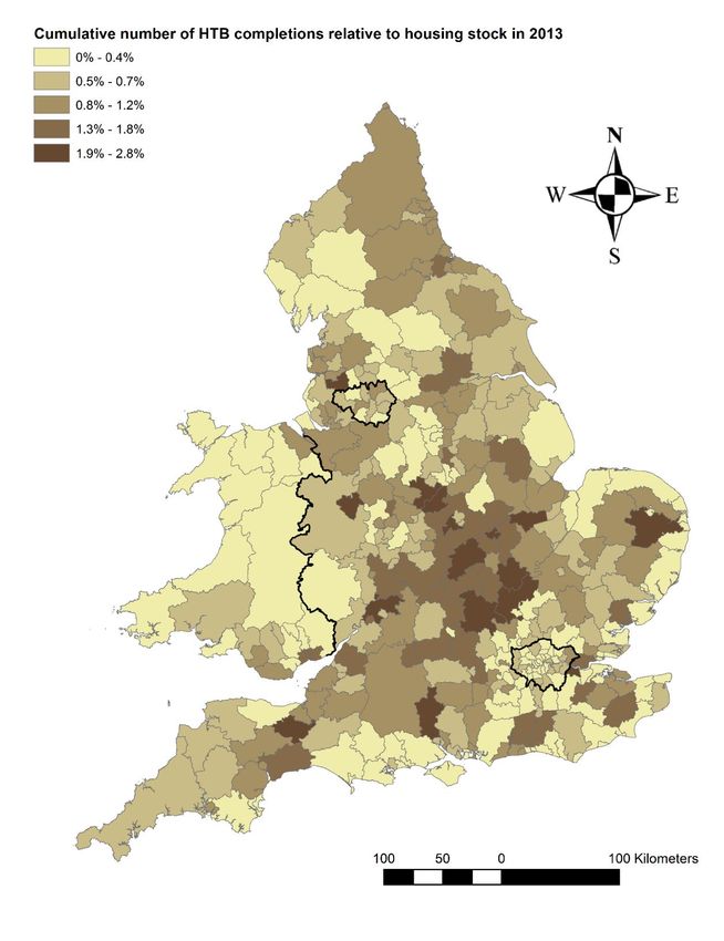
financial data from Orbis. This list includes residential developers, commercial developers and
construction companies.

3.2. The Role of Local Supply Conditions

Below, we report separate estimates of the impact of the generosity of HtB schemes obtained
from a sample of properties near the GLA boundary, and a sample of properties near the
English/Welsh. We choose these two areas because they both provide an ideal quasi-natural
setting to identify the economic effects of HtB. We also report estimates using the area near the
Greater Manchester boundary for our placebo tests, as the same generosity of the English HtB
scheme does not change at that boundary.

One crucial difference between our two focal areas – the area near the GLA boundary and the
area near the English/Welsh border – is that the former has overall vastly less responsive supply,
driven by both, tighter local planning regulations and a relative scarcity of undeveloped
developable land. As shown above, theory suggests that the positive impact of HtB on house
prices should be much larger – and the positive impact on new construction much smaller – in
the area near the GLA boundary.

In order to illustrate the differences in supply conditions between the areas, we employ a
number of measures that capture long-term housing supply constraints. These measures are the
share of land designated as green belt (provided by the Ministry of Housing, Communities and
Local Government), the average planning application refusal rate taken over the period from
1979 to 2008, the average share of developed developable land, and the average elevation range
(all derived from Hilber and Vermeulen, 2016). We calculate these measures for the three areas
employed in our analysis using Local Planning Authority (LPA)-level data and LPA surface
areas as weights.14

Table 3 (rows 1 to 4) illustrates the differences in supply conditions between the three areas.
The most striking difference between the two focal areas lies in the share of ‘green belt’ land.
Land in green belts is typically off limits for any development (residential or commercial) and
thus represents a ‘horizontal’ supply constraint. This share is 66.5% for boroughs along the
boundary of the GLA but only 3.8% for English boroughs along the English/Welsh border.
Another measure to capture physical supply constraints is the share of developable land already

14
 We do not currently have data for LPAs on the Welsh side of the English/Welsh border. We expect that the
differences between the GLA and the English/Welsh border area will be even more striking when taking account
of the data from the Welsh LPAs.

 11

developed. This share is 27.6% for boroughs along the GLA boundary but only 6.3% for
English boroughs along the English/Welsh border.

The arguably quantitatively most important long-term supply constraint are restrictions
imposed by the British planning system (Hilber and Vermeulen 2016). The weighted average
of this refusal rate is 35.6% for boroughs along the GLA boundary and 27.2% for English
boroughs along the English/Welsh border.

While the area near the English/Welsh border is subject to greater topographical (slope related)
supply constraints, Hilber and Vermeulen (2016) demonstrate that these constraints, while
statistically significant, are quantitatively unimportant in explaining local price-earnings
elasticities.

Lastly, it is important to point out that the area near the GLA boundary is not only characterized
by vastly more restrictive supply conditions, but these constraints are also significantly more
binding in practice, simply because aggregate housing demand there is much stronger. To
illustrate this point, consider a ten-story height restriction in the heart of a superstar city such
as London and compare it to the same constraint in the desert. The restriction is extremely
binding in the former location, while completely irrelevant in the latter.

To explore the differences in supply responsiveness across the three areas further, we employ
the estimated coefficients from Hilber and Vermeulen (2016) to compute an implied house
price-earnings elasticity. Table 3 (rows 5 and 6) reports our estimated elasticities based on these
coefficients. Using the OLS estimates, we find that the price-earnings elasticity along the GLA
boundary (0.40) is higher than that of the area along the Greater Manchester boundary (0.28),
which in turn is higher than the elasticity near the English/Welsh border (0.25). As two of the
three supply constraints measures employed in their estimation, refusal rate and share
developed land, are likely endogenous, we employ the instrumental variable strategy proposed
in Hilber and Vermeulen (2016). This provides exogenous variation in our supply constraint
measures, which we use to re-compute the unbiased price-earnings elasticities. The rank order
remains unchanged. The GLA has again the highest elasticity (0.21) followed by Greater
Manchester (0.16) and the English/Welsh border area (0.13).

The higher price-earnings elasticity along GLA boundary suggests that, due to local supply
constraints, housing prices respond more strongly to a given change in local housing demand.
This also suggests a lower supply price elasticity in the GLA boundary area. In the next section,

 12

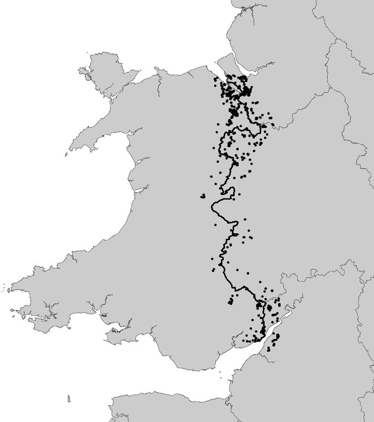
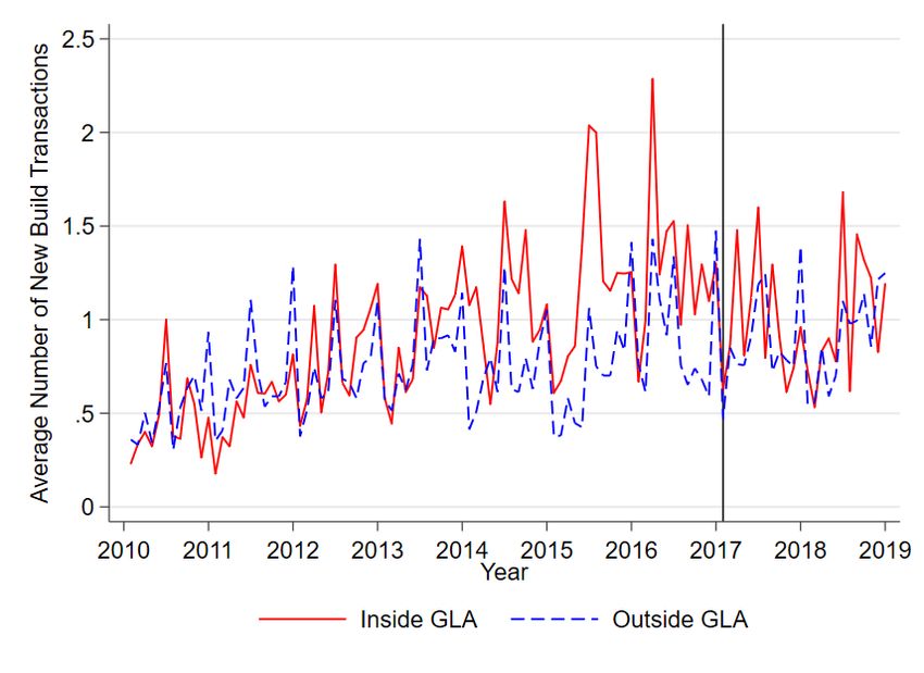
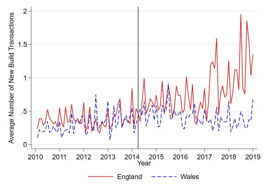
we outline our identification strategy and discuss how we measure the impact of HtB on house
prices and construction activity.

3.3. Identification Strategy and Empirical Specifications

Our empirical strategy is designed to test the impact of HtB on housing construction and house
prices. We exploit spatial differences in the intensity of the HtB policy. As mentioned above,
HtB Wales was rolled out nine months later than in England and offered a government-backed
loan for the purchase of new build properties under £300,000 (£600,000 in England). There
were also differences in the intensity of the HtB policy between the GLA and its surroundings,
starting in 2016. In this case, the difference lies in the size of the government-backed loan
available to households. London-HtB offers loans of up to 40% of a new build’s value, while
this figure is 20% elsewhere (i.e., outside the GLA boundary). We exploit these regional policy
differences in a Difference-in-Discontinuities design combining time variation in prices and
new build construction with local variation in policy intensity around the regional boundaries.

The samples of new build properties used in the analyses of prices and construction effects near
the GLA boundary and the English/Welsh border are illustrated in Figures 1 and 2,
respectively.15 Our boundary approach is meant to ensure that we are comparing properties
affected by similar economic and amenity shocks, as compared to a standard Difference-in-
Differences strategy that simply takes whole regions as control groups. The identifying
assumption in both cases can be likened to the typical assumption of parallel trends: in the
absence of the policy, prices and construction on either side of the boundary would have
followed a parallel evolution over time. Figures 3 and 4 depict the evolution of house prices at
both sides of the GLA boundary and English/Welsh border, respectively, and indicate that
prices moved in parallel prior to the implementation of the policy.16 Figures 5 and 6 depict the
average number of units built by ward at the GLA boundary and English/Welsh border,
respectively. Again, we see that the evolution of building activity followed reasonably parallel
trends prior to the implementation of the policy.

In addition to studying the effect of the policy on prices and construction activity, we also
estimate the impact on HtB on developers’ profits, and document evidence of substantial

15
 Appendix Figure A1 depicts the corresponding map for our placebo sample of new build sales near the Greater
Manchester boundary.
16
 The price index is constructed by estimating a linear regression of log prices on property characteristics (property
type dummies for detached, semidetached and terraced properties, property size, a leasehold dummy, measures of
energy efficiency) and postcode fixed effects. The lines in Figures 3 and 4 correspond to time dummies included
in that specification.

 13

bunching of new build property prices around the eligibility thresholds for England (£600,000)
and Wales. These specific analyses further clarify developers’ responses to the policy.

3.3.1. Specification: Impact of Help to Buy on House Prices

The HtB policy is meant to operate as a relaxation of households’ credit constraints. Hence, it
can lead to an increase in demand for new builds, and as a result, to an increase in the price of
new builds. To test this, we use observed transactions of new build units located near the
boundary of the GLA and the English/Welsh border in two Difference-in-Discontinuities
analyses. We conduct both exercises separately. To estimate the magnitude of these differences
in our Difference-in-Discontinuities framework we estimate:

ln( ) = + × + + ′ + ′ × + × + (3)

where indexes individual properties, j indexes the (ward-level) neighborhood, p indexes the
postcode (within a ward), indexes the month, and y indexes the year. The variable is a
dummy that takes value 1 in the region with a more generous HtB policy (i.e. inside the GLA
or on the English side of the English/Welsh border), and the variable represents a dummy
taking value 1 if individual transaction occurs after the difference in policy takes place. A
vector of postcode fixed effects is represented by , is a set of (year-month) time dummies,
 is a set of individual housing characteristics, and are neighborhood characteristics at the
ward level (from the 2011 Census) interacted with year dummies .

After we control for postcode fixed effects, we include the distance to the boundary interacted
with year dummies to account for potential time varying shocks that differ spatially.17 We
estimate this equation by OLS, clustering standard errors at the postcode-level to account for
potential spatial correlation in local price shocks. This is estimated on properties within a
bandwidth around the corresponding boundary. In the case of the London HtB, we use a 5km
bandwidth around the GLA boundary. We use a 10km bandwidth around the English/Welsh
border. In the robustness checks section, we show that our results are robust to alternative
bandwidth choices.

Our parameter of interest is . It measures the effect of differences in the intensity of the HtB
policy on the price of new build properties.

3.3.2. Specification: Impact of Help to Buy on Housing Construction

17
 In an alternative specification, we omit the postcode fixed effects and control flexibly for distance to the
boundary by estimating different linear terms in the distance, specified separately on either side.

 14

The government’s equity loan is available only for the purchase of new build units. In this way,
the government attempts to ensure the policy triggers additional residential construction. In
order to test whether this is the case, we estimate the effect of differences in the intensity of the
policy on construction activity. We again use a Difference-in-Discontinuities specification.
This exercise is conducted by aggregating new build counts at the ward level for every month.
We estimate:

 = + × −12 + + ′ × + × + (4)

where indexes wards, indexes months, and y indexes years. The dependent variable is
now , which can represent either the number of new build transactions in ward 
and period , or a dummy taking value 1 if there are any new build sales in ward and period .
The variable is a dummy taking value 1 in the area with a more generous HtB policy (i.e.,
inside the GLA boundary or on the English side of the English/Welsh border), and the variable
 −12 represents a dummy that takes value 1 if transactions in ward occur after the
difference in policy arises. The variable is lagged by twelve months to account for the likely
delayed response of construction to the policy shock.18 We include a set of ward fixed effects,
represented by and time fixed effects .19 are neighborhood characteristics (from the
2011 Census) interacted with year dummies . In addition to controlling for ward fixed effects,
we include the distance to the boundary interacted with year dummies to account for potential
time varying shocks that differ spatially. In all specifications we cluster standard errors at the
ward level to account for potential spatial correlation. We estimate our specification using
observations within 5km of the boundary in the case of the London GLA, and 10km in the case
of the English/Welsh border.

Our parameter of interest is , which measures the effect of differences in the intensity of HtB
on new construction. The differences in intensity are not the same across the English/Welsh
border and across the GLA boundary. Therefore, we obtain separate estimates for these two
exercises.

3.3.3 Help to buy and Developers’ Financial Performance

As indicated in Proposition 2, the increase in demand for newly built housing induced by HtB
should positively impact the financial performance of firms participating in the scheme. The

18
 As a robustness check, we estimate a contemporaneous specification. Construction lags in the UK tend to be
long by international standards, often in excess of 12 months.
19
 We also provide estimates that are obtained by controlling flexibly for distance to the boundary, omitting ward
fixed effects.

 15

policy should induce an increase in revenue of existing developers. 20 Moreover, barriers to
entry and imperfect competition in the housing production and land markets imply that the
policy should translate into increased profits. This, however, depends on whether the increase
in revenues is neutralized by an increase in the costs of land after the implementation of the
policy.21 Uncovering how HtB affected the performance of developers can therefore identify
some of the beneficiaries of this policy.
To study this empirically, we use our developer dataset, covering 84 large British developers
and construction companies. The dataset includes information on developers’ financial
performance and, crucially, on the participation of these firms in HtB. We use our dataset to
compare how the change in the performance of firms before and after 2012 varied with their
participation in the scheme. For this purpose, we estimate a fixed effect model specified as:

 = × + + + (5)

 is an indicator of various measures of financial performance for
developer in year . We look at turnover (i.e. total revenues), gross profits, net profits before
taxes, the difference between gross and net profits, and the salary cost of employees. The latter
two variables are crude proxy measures for the pay packages of the senior management. The
measure captures whether a developer participates in the program. We use two different
definitions of this variable depending on the information available and therefore conduct the
analysis on two separate samples. Our intensity sample consists of the 30 developers, for which
we know the fraction of the units produced that were sold under the HtB scheme. We average
this figure over time to obtain a time-invariant average fraction of units per developer. Our
second definition of is based on the registry of developers in regional HtB offices across
the country. In this case, the variable is a dummy taking value 1 if the developer is included in
the registry. The information on registrations is available across a larger group of firms, so we
can estimate this specification for our larger Difference-in-Differences sample of 84
developers. Variable is a variable taking value 1 after 2012. Finally, is a developer
fixed-effect and represents a set of year dummies.

Estimates of will measure the impact of the policy of firms and revenues under the
assumption that unobservables are uncorrelated with × conditional on
individual and year effects. Because firms actively self-select into the program, the identifying

20
 The increased supply could in principle be taken up exclusively by new entrants. Yet the presence of economies
of scale in housing production and the learning curve required to navigate the British planning system mean the
volume of new entrants will probably be very small.
21
 In our model, this is ruled out because land is owned by developers, so land rents are included in profits.

 16

assumption requires that the difference in performance between firms that self-select into the
scheme and those that do not is fixed over time. That is, we assume other shocks to performance
during the 2010-2018 period are uncorrelated with program participation.

3.3.4. Bunching Analysis

The English HtB policy is only available for properties purchased under 600,000 GBP. We can
use this threshold to study bunching of property sales close to this price level. In doing so, we
apply some of the methods recently developed in Chetty et al. (2011), Kleven (2016) and Best
and Kleven (2017). The purpose of this analysis is two-fold. First, it allows us to test whether
HtB induced a change in the type of properties supplied by developers. In addition, a bunching
analysis provides an alternative method to study the effect of the policy on building volumes.

We first document that indeed there is substantial bunching at the £600,000 price threshold.
Next, we construct a counterfactual price distribution for new builds using information on sales
excluding the region around the bunching thresholds. Following Kleven (2016), we estimate
this counterfactual distribution by calculating the number of new build transactions in 5000
GBP bins and use these to estimate:
 
 = ∑3 =0 + ∑ ∈ 1 { ∈ ℕ} + (6)

where indexes price bins and indexes time. The dependent variable measures the number
of new build transactions in bin at time . The first two sums provide an estimate of the
counterfactual price distribution. The first sum is a third-degree polynomial on the distance
between price bin l and the cutoff of £600,000. The second sum estimates fixed-effects for
round numbers, with ℕ representing the set of natural numbers and =
{5000, 10000, 25000, 50000} representing a set of round numbers. We estimate this equation
with data for new build transactions in England taking place after April of 2013 (the
introduction of HtB in England). We then obtain differences between this estimated
counterfactual distribution and the observed distribution of prices to estimate bunching effects
induced by HtB.

The difference between the size of the spike just under the threshold and the gap just after the
threshold can be used to estimate the size of the local effect of HtB on new building activity.
This can be driven by changes in the types of properties sold after accounting for local shifting
in prices induced by the policy.

3.4. Main Results

 17

3.4. 1. Visual Evidence of Boundary Discontinuity

We first provide a series of graphs that illustrate our main results. Figure 7 represents the prices
for newly built units at different distances from the GLA boundary. Positive distances
correspond to locations inside the GLA, while negative distances refer to locations outside of
this area. Circles depict the mean value of new build house prices for 500-meter-wide distance
bins with the size of each circle being proportional to the number of observations in that bin.
Lines in both panels represent fitted values from 2nd order polynomials estimated separately on
each side of the boundary. Gray bands around them represent 95% confidence intervals.22
Panels A and B illustrate results before and after the introduction of London HtB, respectively.
Comparing both panels, we find that a discontinuity in prices at the boundary emerges after the
implementation of London’s HtB. We interpret this as evidence that differences in the size of
available equity loans at the boundary led to a significant and positive effect on the price of
newly built properties within London. We test this formally in Section 3.4.2.

Figure 8 illustrates our results for the new build price effect at the English/Welsh border. Circles
depict the mean value of house prices for 1000-meter-wide distance bins. As above, solid lines
represent 2nd degree polynomials estimated on both sides of the boundary. 23 In this case,
however, we do not observe a spatial discontinuity of house prices in either Panel A or B.
Hence, the difference in the scheme at the border – the eligibility price threshold is twice as
large in England as in Wales – did not generate an appreciable difference in new build prices.

We conduct a similar exercise looking at changes in construction volumes at these boundaries
before and after the corresponding changes in HtB. Results are illustrated in Figures 9 and 10.
The former shows construction as measured by new build sales near the GLA boundary with
Panels A and B corresponding to the periods prior and post implementation of London HtB,
respectively. We do not find a spatial discontinuity in homebuilding at the London boundary in
either period. Figure 10 shows results for the English/Welsh border before and after the English
HtB policy was implemented. In this case, we find a clear discontinuity emerging in Panel B,
indicating more building took place on the English side of the boundary after the policy was
introduced.

22
 We report 2nd degree polynomials in these figures because they yield a lower Akaike Information Criterion
statistic than 1st degree polynomials. Appendix Figure A2 reports results when using linear equations on either
side of the boundary.
23
 Appendix Figure A3 reports results when using a linear polynomial.

 18

Finally, we conduct a placebo experiment using properties sold around the Greater Manchester
boundary to test whether any spatial discontinuities in prices emerge after the introduction of
London HtB in 2016. Note that the intensity of the policy is identical inside and outside the
Manchester boundary. Results are provided in Figure A4 in the Appendix. As expected, we
observe no discontinuity in prices at the boundary before or after the London HtB policy was
put in place.

Overall, these graphs indicate that more generous versions of the policy triggered a price
response in the supply inelastic areas around London. Conversely, the policy generated a
quantity response in the relatively supply elastic areas around the English/Welsh border. This
is in line with the intuition that price or quantity responses to shifts in demand depend on the
shape of the supply curve, as illustrated in the theoretical framework provided in Section 2.2.
In the following two sections, we present reduced-form estimates for the magnitudes of these
effects.

3.4.2. Effect of HtB on House Prices

Table 4 summarizes the results from estimating equation (3) using the sample of transactions
of new build properties within 5 kilometers from the GLA boundary. Different sets of covariates
are included sequentially from columns 1 to 5. Column 1 controls for time effects and
independent linear terms in distance of each property to the GLA boundary. Column 2 adds a
vector of housing characteristics such as total floor area, type of the property, and tenure of the
property. Column 3 adds postcode fixed effects. In column 4 we include neighborhood
characteristics from the census interacted with year effects. Finally, in column 5, we allow for
heterogeneous spatial price trends by controlling for interactions between distance from the
GLA boundary and year dummies. Our preferred specifications are controlling for property
characteristics. The standard errors in all specifications are clustered at the postcode level to
allow for a degree of spatial correlation in the error term.

The resulting estimates show that London’s HtB policy increased the price of newly built
houses inside the GLA by between 4.5% and 6.4% depending on the specification, with 4 out
of 5 estimates being significant at the 1% level. The average property price in this sample is
£394,703, so this finding suggests that homebuyers are paying £24,393 more to buy newly built
properties inside the GLA because of London’s HtB (compared to the less generous English-
version of the scheme). In Section 3.7, we compare this effect to that which would result from
the implicit interest subsidy provided by the equity loan granted by the scheme.

 19

Table 5 summarizes the results from estimating equation (3) for the sample of properties around
the English/Welsh border. Again, we successively include additional controls from columns 1
to 5. Once we control for postcode fixed effects, we observe no significant effect of the policy
on the price of new build sales. The point estimates in columns 3 to 5 are positive but small,
ranging between 1.7 and 2.5%, and not statistically significant, with p-values above 0.37 in all
specifications.

These estimates confirm the results reported in the graphical analysis provided in Section 3.4.1
and are also in line with the predictions highlighted in our theoretical framework. As land
supply is relatively inelastic near the GLA boundary, the shift in demand induced by HtB is
capitalized into prices. Near the English/Welsh border, where developable land is available, the
response is more likely to happen in quantities rather than prices. Naturally, this hypothesis is
testable; we estimate the effect of HtB on housing supply in the next section.

3.4.3. Effect of HtB on Housing Construction

Table 6 summarizes the results from estimating equation (4) for the sample including all wards
within 5 kilometers of the GLA boundary. We define the post-HtB period as extending from
February 2017 to December 2018, – starting one year after the implementation of London’s
HtB – to allow for a one-year construction lag. From Table 6, we observe that London’s HtB
did neither have a significant effect on construction volumes nor on the probability that any
newly built property was sold in a ward. Coefficients are insignificant and small in all
specifications, indicating that the increase in the size of available equity loans at the boundary
did not lead to an increase in housing supply.

In Table 7, we provide estimates of equation (4) for wards around the English/Welsh border.
As above, the post-treatment period is defined as starting one year after the introduction of the
English HtB-scheme. We find a significant and positive effect of HtB on housing construction
in all specifications. Our estimates suggest that the higher eligibility threshold on the English
side of the boundary increased the number of new build transactions at each ward by 0.42 on
average, and the propensity for any new build construction at each ward by 7.8%. These results
are consistent with the predictions from our theoretical framework that indicate that HtB has
differential effects in London and the areas around Wales as a consequence of differences in
supply conditions in the two areas.

3.4.4. Effect of HtB on Financial Performance of Developers

 20