Chlorophyll fluorescence as a biological feedback signal - Linnéa Ahlman thesis for the degree of doctor of philosophy
←
→
Page content transcription
If your browser does not render page correctly, please read the page content below
thesis for the degree of doctor of philosophy

     Chlorophyll fluorescence as
     a biological feedback signal

              Linnéa Ahlman

       Department of Electrical Engineering
        Chalmers University of Technology
           Gothenburg, Sweden, 2021
Chlorophyll fluorescence as a biological feedback signal

Linnéa Ahlman
ISBN 978-91-7905-561-5

Copyright c 2021 Linnéa Ahlman
All rights reserved.

Doktorsavhandlingar vid Chalmers tekniska högskola
Ny serie nr 5028
ISSN 0346-718X

Department of Electrical Engineering
Division of Systems and Control
Chalmers University of Technology
SE-412 96 Gothenburg, Sweden
Phone: +46 (0)31 772 1000
www.chalmers.se

This thesis has been prepared using LATEX
Printed by Chalmers digitaltryck
Gothenburg, Sweden, 2021
To my beloved
Abstract
The use of light emitting diodes (LEDs) instead of traditional high pressure
sodium lamps, in greenhouses and indoor growing facilities, enables tuning
and optimization of both light intensity and light spectrum. This opens for
an energy saving potential not possible otherwise. Furthermore, such con-
trollable lamps can be used to generate low intensity light excitations, which
cause changes in the plants’ chlorophyll fluorescence (ChlF). Analysis of these
changes can then be used for plant diagnosis. We have conducted such ex-
periments on plants to evaluate if and how proximal sensed ChlF, measured
on canopy level, can be used as a biological feedback signal for spectrum
optimization, stress detection, and for light intensity optimization.
   We found that steady-state ChlF have a strong correlation with short term
photosynthesis and can be used for estimation of relative efficiency of different
LED colors with respect to each other. We did not find significant changes
in the relative efficiencies when light intensity or spectrum was changed, as
was initially hypothesized. However, the method can still be applicable for
spectrum calibration, as the efficiencies of different LED colors vary individ-
ually as the diodes degrade with time and they also vary to different degree
depending on the operating temperature.
   Experiments on abiotically stressed plants (drought, salt, and heat) showed
that variations in the dynamics of the ChlF signal can be used to classify
plants as healthy or unhealthy. Experiments with the root infection Pythium
ultimum indicated that severe infection is detectable. This is promising as it
by its nature is hard to detect without harvesting. More research is needed
though, to statistically verify if this, and other biotic stress factors can be
detected, and if so, how severe the infection must be.
   Fast ChlF gain, defined as the amplitude of the ChlF signal caused by
light pulses with a high frequency and a low intensity, was found to have a
concave shape with respect to light intensity. Furthermore, the light intensity
corresponding to the maximum of the fast ChlF gain coincide with the light
level where the photosynthetic rate starts to saturate, which in some sense can
be regarded as an optimal light level for efficient growth. Hence, we suggest
the use of an extremum seeking controller to force the light intensity level to
this point and demonstrates how this works in a simulation study.

Keywords: Fluorescence gain, dynamics, LED, classification, ESC, light
spectrum, greenhouse lighting control, indoor farming, basil, cucumber, lemon
balm, lettuce, strawberries, abiotic stress, biotic stress, Pythium ultimum,
powdery mildew Podosphaera aphanis.

                                                                                i
ii
Acknowledgments
It literally required blood, sweat, and tears. Now, when approaching the end
of this PhD journey it looks like it was worth it! First of all, I would like to
thank my supervisor/examiner/boss (and unofficial therapist), Prof. Torsten
Wik. Thank you for your support, encourage, and the will of sharing your
deep knowledge.
   I would also like to thank my former colleague Anna-Maria Carstensen, who
paved the way in this interdisciplinary area, making my way much smoother.
Thank you Daniel Bånkestad for the rewarding collaboration throughout the
years. Finally, I want to thank all present and former colleagues at the de-
partment, for all interesting, deep, superficial, and fun conversations in the
lunchroom.
   When I started as a PhD student, I was newly married. Since then, all the
work summarized in this thesis was done, but not only that. Furthermost,
we have had our three adorable kids, and we have survived some intense
and sleepless years when the twins were babies. Above all, we did that and
everything else, as a team. I look forward to celebrate our ten–year wedding
anniversary next year. Marcus, thank you for your patience, I love you!

                                                               Linnéa Ahlman
                                                               Sävedalen, 2021

                                                                              iii
iv
List of publications
This thesis is based on the following publications:

[A] Linnéa Ahlman, Daniel Bånkestad, Torsten Wik, “Using chlorophyll a
fluorescence gains to optimize LED light spectrum for short term photosyn-
thesis”. Computers and Electronics in Agriculture, 2017.

[B] Linnéa Ahlman, Daniel Bånkestad, Torsten Wik, “LED spectrum opti-
misation using steady-state fluorescence gains”. Acta Horticulturae, 2016.

[C] Linnéa Ahlman, Daniel Bånkestad, Torsten Wik, “Relation between
changes in photosynthetic rate and changes in canopy level chlorophyll flu-
orescence generated by light excitation of different LED colours in various
background light”. Remote sensing, 2019.

[D] Linnéa Ahlman, Daniel Bånkestad, Sammar Khalil, Karl-Johan Bergstrand,
Torsten Wik, “Stress detection using proximal sensing of chlorophyll fluores-
cence on canopy level”. AgriEngineering, 2021.

[E] Linnéa Ahlman, Daniel Bånkestad, Torsten Wik, “Tracking optimal
plant illumination using proximal sensed chlorophyll fluorescence gain”. Manuscript,
2021.

                                                                             v
vi
Contents

Abstract                                                                                                                i

Acknowledgements                                                                                                      iii

List of publications                                                                                                   v

I   Introductory chapters                                                                                              1

1 Introduction                                                                                                         3
  1.1 Aims & Objectives . . . . . . . . . . . . . . . . . . . . . . . . .                                              4
  1.2 Thesis outline . . . . . . . . . . . . . . . . . . . . . . . . . . . .                                           5

2 Preliminaries                                                                                                        7
  2.1 Photobiology . . . . . . . . .      .   .   .   .   .   .   .   .   .   .   .   .   .   .   .   .   .   .   .    7
       Measuring light . . . . . . . .    .   .   .   .   .   .   .   .   .   .   .   .   .   .   .   .   .   .   .    7
       Ambient light . . . . . . . . .    .   .   .   .   .   .   .   .   .   .   .   .   .   .   .   .   .   .   .    8
       Photosynthesis . . . . . . . .     .   .   .   .   .   .   .   .   .   .   .   .   .   .   .   .   .   .   .    9
       Chlorophyll a fluorescence . .     .   .   .   .   .   .   .   .   .   .   .   .   .   .   .   .   .   .   .   14
  2.2 Growth lighting . . . . . . . .     .   .   .   .   .   .   .   .   .   .   .   .   .   .   .   .   .   .   .   15
       High intensity discharge lights    .   .   .   .   .   .   .   .   .   .   .   .   .   .   .   .   .   .   .   15
       Fluorescent lights . . . . . . .   .   .   .   .   .   .   .   .   .   .   .   .   .   .   .   .   .   .   .   16
       Light emitting diodes . . . . .    .   .   .   .   .   .   .   .   .   .   .   .   .   .   .   .   .   .   .   16
       Choice of light source . . . .     .   .   .   .   .   .   .   .   .   .   .   .   .   .   .   .   .   .   .   17

                                                                                                                      vii
2.3 Extremum seeking control . . . . . . . . . . . . . . . . . . . . . 17
Sinusoid perturbation ESC . . . . . . . . . . . . . . . . . . . . 18
Constant stepping ESC . . . . . . . . . . . . . . . . . . . . . . 20
3 Research areas 21
3.1 Light spectrum optimization . . . . . . . . . . . . . . . . . . . . 21
3.2 Stress detection . . . . . . . . . . . . . . . . . . . . . . . . . . . 23
3.3 Light intensity optimization . . . . . . . . . . . . . . . . . . . . 24
Ongoing experiments . . . . . . . . . . . . . . . . . . . . . . . . 26
4 Summary of included papers 29
4.1 Paper A . . . . . . . . . . . . . . . . . . . . . . . . . . . . . . . 29
4.2 Paper B . . . . . . . . . . . . . . . . . . . . . . . . . . . . . . . 30
4.3 Paper C . . . . . . . . . . . . . . . . . . . . . . . . . . . . . . . 30
4.4 Paper D . . . . . . . . . . . . . . . . . . . . . . . . . . . . . . . 31
4.5 Paper E . . . . . . . . . . . . . . . . . . . . . . . . . . . . . . . 32
5 Concluding remarks and future directions 33
References 37
II Papers 43
A Using chlorophyll a fluorescence gains to optimize LED light spec-
trum for short term photosynthesis A1
B LED spectrum optimisation using steady-state fluorescence gains B1
C Relation between changes in photosynthetic rate and changes in
canopy level chlorophyll fluorescence C1
D Stress detection using proximal sensing of chlorophyll fluorescence
on canopy level D1
E Tracking optimal plant illumination using proximal sensed chloro-
phyll fluorescence gain E1
viiiPart I
Introductory chapters
1CHAPTER 1
Introduction
Indoor farming enables production of fresh vegetables in urban areas, which
is expected to be increasingly important as the world’s urban population is
growing. In such regions, vertical farms, or top roof gardens, can be effi-
cient ways of utilizing the area and producing food close to customers. Huge
amounts of resources are brought into urban areas, and huge amounts of waste
are produced. However, much of the waste can be a resource for urban farm-
ing, such as wastewater, heat, food and garden waste, CO2 -enriched air from
offices and factories etc [1].
Another advantage with indoor farming is the possibility of having a high
level of control. This opens for optimization of growth conditions to maximize
yield. It is also less, or not at all, affected by weather conditions, neither
seasonal variations nor occasional extreme weather conditions, thus paving
the way for a stable and predictable food production.
Productive dense indoor farming though, requires efficient artificial light
sources. The lamps traditionally used in greenhouses, i.e., high pressure
sodium (HPS) lamps, are not well suited for this purpose. They produce
a lot of radiant heat and, hence, close distance between lamps and plants is
not possible. Furthermore, they have a fixed spectrum and are not well suited
for frequent turning on and off, meaning that tuning of spectrum or intensity
is not applicable. However, the rapid development of light emitting diodes
(LEDs) has led to the possibility of both proximal distance between lamps and
3Chapter 1 Introduction
plants, and control of both spectrum and intensity. Hence, the LED lighting
opens for a more efficient lighting economy since spectrum and intensity can
be optimized for maximal yield and minimal energy consumption.
1.1 Aims & Objectives
The experiments conducted in the work behind this thesis aims at contributing
to the work of finding optimal growth conditions for greenhouses or indoor
farming. More specifically, our approach has been to use the chlorophyll
fluorescence, ChlF, emitted from the plants as a response to deliberate changes
in the light intensity they receive, as a biological feedback for improved farming
and resource economy.
The general setup has been to use commercial greenhouse LED-lamps to,
not only supply growth light, but also to generate the deliberate superimposed
light excitations, and then measure the variations in ChlF, from above, on
canopy level. The work can be divided into three different research areas:
Spectrum optimization, Stress detection and Intensity optimization.
In the Spectrum optimization, the main aim was to evaluate the possi-
bility of using fluorescence gains as a biological feedback for spectrum opti-
mization of plant growth. This was investigated, by experiments presented in
Paper A, B, and C, to answer the questions:
• Can remotely measured steady-state fluorescence be a sufficiently good
measure of photosynthetic rate for this purpose?
• Does the magnitude of the fluorescence gains, caused by light excitations
of different colors, change relative to each other when the illumination
intensity and/or spectrum are changed and, further, do they depend on
plant species?
The work in the other two areas were part of a prestudy for a sensor de-
velopment project, with the goal of developing a cheap and relatively simple
fluorescence sensor as a monitoring tool to be used in greenhouses.
In the Stress detection work we investigated the possibility of extract-
ing plant health information in the fluorescence signal, and the results are
presented in Paper D. We then tried to answer the question:
• Can different abiotic as well as biotic stress factors be detected from the
dynamics of the remotely sensed chlorophyll fluorescence signal gener-
ated by low intensity excitations?
Finally, in the Intensity optimization work we investigate a new method
to find the optimal light intensity online. From previous experiments we
41.2 Thesis outline
had measurements showing that there is a peak in the fluorescence gain as a
function of light intensity. Based on this we investigated:
• Does the light intensity that corresponds to a peak in the fluorescence
gain also corresponds to the, in some sense, optimal growth light inten-
sity?
• How should a controller that controls the light towards this point be
implemented?
The answer to the first question is investigated by experiments and then, in
simulation, we show how an extremum seeking controller can be effectively
used for the proposed control task. The results are summarized in Paper E.
1.2 Thesis outline
The first part of this thesis has the purpose of introducing the reader to the
areas covered to facilitate the reading of the appended papers. In the next
chapter some background knowledge regarding photobiology, growth lighting
and extremum seeking control is given, and in Chapter 3 the three research
areas are introduced. Further on, in Chapter 4 the included papers are summa-
rized and Chapter 5 gives concluding remarks and indicates future directions
of research. Finally, the five papers are appended as a second part of this
thesis.
5CHAPTER 2
Preliminaries
2.1 Photobiology
Measuring light
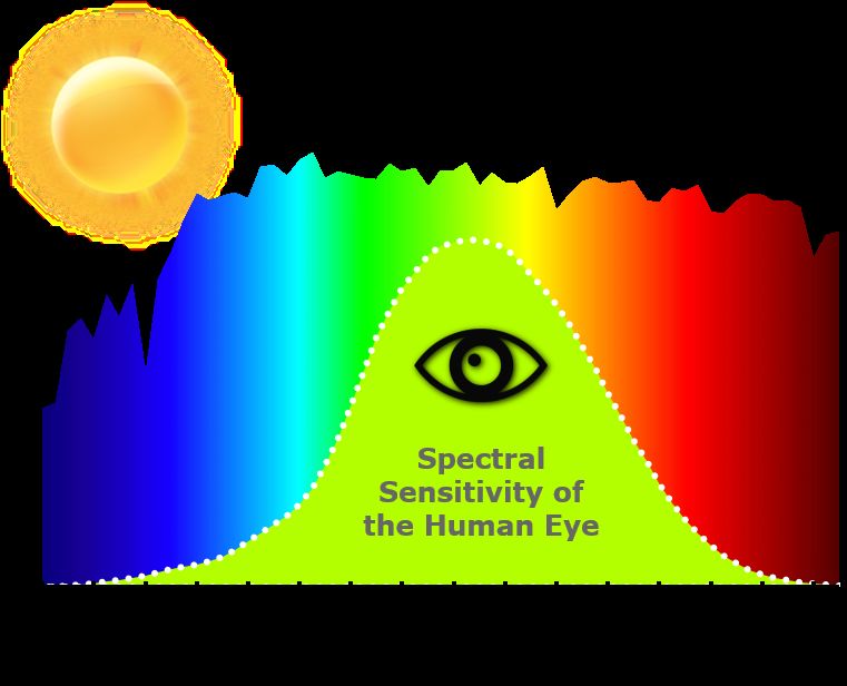
The spectrum visible for the human eye is within 380 to 750 nm, but the sen-
sitivity to various wavelengths differs a lot (Figure 2.1). We are most sensitive
to green/yellow light and gradually less sensitive for decreasing wavelengths
into the blue area and increasing wavelengths into the red area. When consid-
ering how bright a light is to a human, this must be taken into consideration.
This is indeed the case when measuring luminous flux, in lumen (lm), which is
the radiant flux weighted according to the human eye’s sensitivity to various
wavelengths. However, the luminous flux is not a relevant quantity for plants.
Instead, it is mainly the number of photons (per area and time) that is of
interest.
The photosynthetically active radiation (PAR) is the flux of photons with
wavelengths 400–700 nm, since that is the light that mostly contributes to
the photosynthesis. Even though the photons within this region contribute to
slightly different degrees, all of them are equally weighted when calculating
the photosynthetic photon flux density (PPFD) having the unit µmol m−2 s−1 .
Moreover, in addition to measuring light in lumen or PPFD, the energy flux,
having the unit W m−2 s−1 , is of interest when regarding the lighting with
7Chapter 2 Preliminaries
Figure 2.1: Rough illustration of human eye’s sensitivity to various wavelengths [2].
respect to the electricity consumed. The energy flux within the PAR wave-
lengths is Z 700
Energy flux = PPFD × E(λ)dλ × NA , (2.1)
400
where NA is Avogadro’s constant, i.e., numbers (of photons) per mole, and
E(λ) is the energy of one photon having wavelength λ, which is given by
hc
E(λ) = , (2.2)
λ
where h is Planck’s constant and c is the speed of light. Since the energy is
inversely proportional to the wavelength, a photon of higher wavelength than
another, has less energy, which means that it will cost less energy to produce
that one, assuming equal electric efficiency.
Ambient light
The amount of ambient light that reaches the earth varies a lot over the
year and with location. Light data collected in Sweden (from SMHI [3], lat-
itude 58.58, longitude 16.15) once every hour during 2016 is presented in
Figure 2.2(a), and a closer look into March 2016 is seen in (b) to illustrate the
variability over a month. The maximum intensity was detected in June, with
almost 1700 µmol m−2 s−1 , while the maximum intensity in December was sel-
dom above 200 µmol m−2 s−1 . Figure 2.3 shows the PAR collected in Spain,
in September 2018. This data set is collected with a sample rate of 2 seconds.
It shows that the light intensity variations can be large, even within second
82.1 Photobiology
scale. This is most pronounced with a clear sky, when mostly direct light is
measured, whereas a cloudy day the light is diffuse and hence the variations
are much smaller.
1200
1700
1500 1000
800
PAR
1000
PAR
600
400
500
200
0 0
Jan Apr Jul Oct Jan Mar 01 Mar 08 Mar 15 Mar 22 Mar 29
2016 2016
(a) Light profile 2016. (b) Light profile in March 2016.
Figure 2.2: Ambient light collected in Sweden 2016 [3]. Data collected with a
sample time of 1 h.
The total amount of light that a plant receives within one day is referred
to as the daily light integral (DLI) and is usually expressed as moles of light
(within PAR) per square meter and day. Figure 2.4 shows the mean value
of DLI each month in Sweden 2016. Let us assume that we have a closed
environment with a lamp emitting 300 µmol m−2 s−1 for 12 h/day. That
would equal
300 µmol m−2 s−1 × 12 h/day × 3600 s/h × 10−6 /µ = DLI 13 mol m−2 day−1 .
If further assuming that 60–70% of the ambient light is transmitted through
the roof of a greenhouse, an ambient DLI of about 20 mol m−2 day−1 is needed
to get the same amount of light as in the indoor example. In 2016, 57% of all
days did not reach that and if excluding the summer months (May-August),
82% of the days did not reach that amount of light. This means that for a
large part of the year it is required to have supplemental light to ensure a high
growth rate.
Photosynthesis
The photosynthesis is the process where light energy is transformed into chem-
ical energy, primarily stored as carbohydrates in the plant. The phenomena
is described in many text books, for example by Lawlor [4], Björn [5], and
Durner [6]. Besides light energy, carbon dioxide and water are consumed to
9Chapter 2 Preliminaries
2000 60
50
1500
40
PAR
DLI
1000 30
20
500
10
0 0
08:00 10:00 12:00 14:00 2 4 6 8 10 12
Sep 22, 2018 Month
Figure 2.3: Ambient light data col- Figure 2.4: The daily light integral
lected in September in (DLI) each month (± std)
Spain, with a sample time in Sweden 2016 [3].
of 2 s. Courtesy of
D. Bånkestad.
form carbohydrates and oxygen, roughly according to
light
6 CO2 + 6 H2 O −−−→ C6 H12 O6 + 6 O2 . (2.3)
The photosynthesis takes place in the plant cell, within an organelle called
chloroplast. The chloroplast is filled with a liquid, the stroma, and contains
stacks of thylakoid membranes. In these membranes the chlorophyll and the
carotenoid pigments are found. These are the pigments that absorb the light
energy in the first part of the photosynthesis, called the light reaction.
In the light reaction, light photons are absorbed by the chlorophyll and
carotenoid molecules, which become excited. The energy absorbed by the
carotenoid is transferred to the chlorophyll molecules. The carotenoid is also
vital for protecting the reaction centers from photodamage [7]. The energy
of the excited chlorophyll molecules is passed to other molecules within the
thylakoid, through the reaction centers called photosystem I (PSI) and II
(PSII). They are connected in series and can be regarded as "electron pumps"
powered by light photons [5]. The energy is eventually used to synthesize ATP
and NADPH (adenosine triphosphate and nicotinamide adenine dinucleotide
phosphate), where the energy is temporarily stored until it is used in the next
step, the dark reaction. In the formation of ATP and NADPH, electrons are
removed from PSII. These are replaced by hydrogen ions which are formed
from the oxidation of water,
2 H2 O → O2 + 4 H+ + 4 e− . (2.4)
102.1 Photobiology
The oxygen produced in this step diffuses out of the chloroplast and eventually
exits the leaf to the air.
The dark reaction takes place in the liquid part of the chloroplast, the
stroma. It both occurs in the dark and in the light, and the driving force
for the reactions is the energy from ATP and NADPH. A series of reactions
ends up in the Calvin cycle, where CO2 is reduced to carbohydrates, as a
biologically stable storage of the energy initially harvested from the sun.
Limiting factors
Figure 2.5 shows a schematic picture of a light response curve, i.e., the rate
of photosynthesis for increasing levels of light intensity. Initially, light is the
limiting factor for photosynthesis and, hence, the rate of photosynthesis in-
creases linearly with increasing light intensity. Then it enters a region where
the increase is not as steep and the light response curve starts to saturate
and, finally, in the region of highest light intensity the rate has saturated.
To determine the optimal illumination level is complex, being a question of
illumination cost and revenue of produce, but in terms of high photosynthesis
and a high light use efficiency the intermediate region probably encloses the
optimum.
40
Rate of photosynthesis
35
30
25
20
15
10
5
10 20 30 40
Light intensity
Figure 2.5: A typical light response Figure 2.6: The rate of photosyn-
curve. thesis at saturating
light (PPFD 1600-
2000 µmol m−2 s−1 ).
Redrawn from data by
Jurik et al. [8].
When light is not the primary limiting factor for photosynthesis, it could
for example be the CO2 concentration or the water availability that is limiting
(cf. Eq. 2.3). In a ventilated greenhouse, the CO2 concentration will be close
11Chapter 2 Preliminaries to the ambient concentration, approximately 400 ppm. However, since CO2 is utilized by plants during the days, the CO2 level may drop to 150-200 ppm in sealed greenhouses in daytime [9], [10]. If the CO2 level drops below 100 ppm the CO2 uptake and hence growth will be completely prohibited [10]. For most crops the saturation point is reached at about 1,000-1,300 ppm under ideal circumstances. Higher levels have little additional positive effects and very much higher would hinder plant growth [10]. Hence, to increase growth, CO2 supplementation or enrichment can be used, for example by rerouting flue gases from a boiler, which is effective if there is need for heating as well. It is important though, to make sure having complete combustion avoiding impurities that are harmful to plants and to humans working there [9]. An- other alternative is liquid CO2 , stored in pressurized tanks that is vaporized through vaporizer units [10]. Moreover, the temperature also affects the growth rate. Higher temper- ature enhance growth, up to a certain limit. Figure 2.6 shows the rate of photosynthesis for different temperatures, measured on bigtooth aspen leaves, in saturating light (1,600-2,000 µmol m−2 s−1 ), for two different CO2 levels in the air (experiments by Jurik et al. [8]). At the low CO2 level (close to ambient condition at the time of the experiment), the temperature optimum was 25 ◦ C, while for the high CO2 level it had shifted to 37 ◦ C. Light quality On atom level the energy absorption (and emission) is quantized, as electrons excites from the ground state to a higher excited state. It is the chlorophyll a and b, and to some extent carotenoid pigments, that absorbs the light for photosynthesis. Figure 2.7 shows the absorption spectra for dissolved chlorophyll a and b, they have one peak in the blue region and one in the red. Figures like this one is probably one reason of the common myth that blue and red light is always to prefer in indoor farming. On molecular level and in vivo, where pigments are tightly packed into protein complex, the absorption occurs instead from a broader spectrum of wavelengths. This is due to vibrational energy and more closely spaced molecular orbitals from which electronic transitions occur [11]. In two large pioneering studies in the 70’s [13], [14], the action spectra of leaves were calculated for a large set of species (22 and 33, respectively) i.e., relative CO2 uptake rate per incident photons, for different wavelengths in intervals of 25 nm. Figure 2.8 shows an example for two of the species (the two ones differing the most from the mean). McCree [13] concluded that the curves had similar shape for all species tested, i.e., one peak in red 12
2.1 Photobiology

                                                                          1

                                           Relative quantum efficiency
                                             [CO2 / incident photon]
                                                                         0.8

                                                                         0.6

                                                                         0.4

                                                                         0.2
                                                                                   Pigweed
                                                                                   Castorbean
                                                                          0
                                                                               350 400 450 500 550 600 650 700 750
                                                                                       Wavelengths [nm]

Figure 2.7: Absorption spectrum for        Figure 2.8: Normalised action spectra
            Chlorophyll a and b, in sol-               for incident quanta for Pig-
            vent. Picture from [12].                   weed and Castorbean. Re-
                                                       drawn from data by Mc-
                                                       Cree [13].

and another one in blue, nevertheless there are species dependent differences.
Note also that the values in the green region are significantly higher than
the absorption spectrum for chlorophyll. When evaluating the growth rate
in vivo the action spectrum will vary further due to increased complexity.
For example, in vivo green light significantly contributes to photosynthesis
and biomass accumulation, especially in the inner and lower leaf layers of the
canopy due to the transmission through the first layers [15].
  The McCree action spectra apply only to the use of narrow wavelength span.
The combined effect of different wavelengths, however, is not necessarily the
sum of the quantum efficiency of individual wavelengths. One example of
this is the enhancement obtained when combining light of wavelengths below
680 nm with light of wavelengths above 680 nm (far-red light). This is called
the Emerson effect [16], which is due to the simultaneous excitation of the
two interconnected photosystems operating in series.
  The quality of the light also affects other aspects of growth. For example,
UV-light (280-400 nm) inhibits cell elongation and can cause sunburn while
far-red (700-750 nm) stimulates cell elongation, influence flowering and ger-
mination (Table 8.1 in [6]). Different plant species are more, or less, sensitive
to light quality. For a review of many studies on this topic, see Paradiso and
Proietti [15], Ouzounis et al. [17], and Olle and Viršile [18].

                                                                                                              13
Chapter 2 Preliminaries
Chlorophyll a fluorescence
Chlorophyll fluorescence is the emission of photons when excited molecules
return to a lower energy level [11]. Most emission at normal temperatures
derives from chlorophyll a, thereby the term chlorophyll a fluorescence [4]. In
solution, chlorophyll a emits almost one third of the absorbed light as fluores-
cence, while in vivo the amount is less than a few percent. The fluorescence is
emitted in the near infrared region, having peak wavelengths around 685 nm
and 740 nm. Figure 2.9 shows an example of (a) an incident light spectrum
using four different diode colors and (b) the corresponding reflection and the
fluorescent light. In the experiments conducted within this thesis, the fluo-
rescence signal is derived from the second peak, illustrated by the red colored
area in the figure.
5 10-3
3
Photon flux [ mol/m2 /s/nm]
Photon flux [ mol/m2 /s/nm]
4 2.5
2
3
1.5
2
1
1
0.5
0 0
400 500 600 700 800 400 500 600 700 800
Wavelength [nm] Wavelength [nm]
Figure 2.9: Left—Incident light spectrum using four diode colours. Right—
Reflected and fluorescent light. The fluorescence signal used in the
experiment in this thesis is derived from the 740 nm-peak.
The probability of a photon being reemitted as fluorescence competes with
the probability of photochemistry and heat re-emission. Hence, fluorescence
emission indirectly contains information about the quantum efficiency of pho-
tochemistry and heat dissipation [19]. This close relationship, between chloro-
phyll fluorescence and photosynthesis, has made fluorescence measurements
an indispensable tool in studying photosynthesis in a wide range of applica-
tions, all the way from measurements on-leaf to remotely, from satellites [11],
[19].
142.2 Growth lighting
2.2 Growth lighting
In this section we give a brief overview of different lighting options that are
common for greenhouse and indoor farming.
High intensity discharge lights
In a high intensity discharge (HID) lamp, an electric current is flowing through
a gas mixture [6]. The gas becomes excited by the electrical energy and emits
photons. The spectral distribution of the light is mainly determined by the
gases involved and the pressure within the lamp [5].
High pressure sodium (HPS) lamps and metal halide (MH) are two of
the most common types of HIDs. Both types are used indoor in growth
rooms as well as in greenhouses. They can deliver high light intensities (500–
1,500 µmol m−2 s−1 ) and they have a long life-time, about 30,000 h for HPS
and 15,000 h for MH [6]. HPS has for long been the most commonly used
type of lamp for greenhouses, due to a high photosynthetic photon flux den-
sity, PPFD, per unit electricity. In Table 2.1 the spectral distribution of the
lamps are presented. Compared to sunlight, HPS has a low light flux in UV,
blue and far red while a high light flux in the green waveband. In addition,
HPS emits a substantial part of the photons at higher wavelengths, outside
the PAR or visible light region, hence, not enhancing the photosynthesis. This
is radiant heat, which heats up the plants. To avoid burning of the plants,
the distance between plants and HPS lamps cannot be too short.
Note that all high-pressure lamps should be handled carefully, due to the
potential risk of explosion.
Table 2.1: Spectral comparison of common horticultural light sources (adapted
from [20]). The illumination is normalised to 100 µmol m−2 s−1 within
PAR (400–700 nm).
Light Sunlight HPS MH Cool White
UV–B (250–350) 2.9 0.2 0.7 0.03
UV–A (350–400) 6.2 0.5 6.7 1.1
Blue (400–500) 29.2 6.5 20.4 24.8
Green (500–600) 35.2 56.6 55.5 52.6
Red (600–700) 35.6 36.9 24.1 22.6
Far–red (700–750) 17.0 4.0 4.0 1.4
15Chapter 2 Preliminaries Fluorescent lights Fluorescent lights are not as intense as HID lights and they have a shorter life-time, typically 5,000–10,000 h. The lamp life-time is also affected by the number of times they are turned on, making them unsuitable for frequent turning on and off. The standard choice for greenhouse growers is cool white fluorescent bulbs. They have an acceptable spectral distribution (Table 2.1) and also the greatest PPFD compared to other fluorescent bulbs. Traditionally they have been extensively used where low light intensity is favorable, for examples for starting seedlings or for simulating spring conditions [6]. Light emitting diodes Light emitting diodes, LEDs, are solid-state light emitting devices. Thereby they can instantly be turned on or off, without requiring warm-up time [21]. Advanced LED lamps combine diodes that generate different wavelengths (from broad-band light to narrow-spectrum), into an array with light peaks at several wavelengths [6]. As each diode can be dimmable individually, either by current or by pulse width modulation (PWM), the spectrum can be varied, making LED lamps suited for control of spectrum as well as intensity. The efficacy, µmol per energy input, of individual diodes varies a lot but generally red and blue LEDs have the highest efficacy, while green diodes have efficacies in the order of 1/2 or 1/4 relatively the most efficient ones [22], [23]. The efficacy has gradually increased over time and now there are com- mercial LEDs (with combined colors) currently providing 3.4 µmol J−1 [24]. The theoretically maximal efficacy, with efficiency 100% W/W, is 3.34 and 5.85 µmol J−1 , for wavelengths 400 and 700 nm, respectively. With current techniques it is estimated that the efficacy of combined red and blue LEDs can reach 4.1 µmol J−1 [25]. LEDs do not burn out like a bulb. The most commonly used life-time metric for LEDs is instead the time when the maximum intensity has been reduced by 30%, which occurs after about 50,000 h [26]. Another difference in comparison with bulbs is that LEDs do not radiate heat directly. However, they do produce heat that must be removed to ensure maximal performance and life-time. This can be done by conduction through a liquid cooling device, or through natural or forced convection, in the latter case by using a fan [6]. Furthermore, the fact that LEDs do not radiate heat directly, opens for the ability to place the lamps in close proximity to the plant tissue. This opens up for intermediate lighting or dense vertical farming, with an increased production per land area. 16
2.3 Extremum seeking control

Choice of light source
During the last two decades it has been debated if and how much the economy
in greenhouses can be improved by replacing the traditional HPS lamps by
LEDs. The main arguments have been that the efficiency of LEDs is higher,
but on the other hand the investment cost is higher, as well as the need of
supplemental heating. The total economy balance is affected by many factors
and the conclusion can differ depending on initial assumptions. Furthermore,
ongoing development of the lamps also change the prerequisites.
   In a study from 2014, Nelson and Bugbee [23] concluded that the energy
efficacy, i.e., produced µmol per energy input, at that time was about the
same, 1.7 µmol J−1 , for the most efficient (1000 W) HPS and LED fixture,
but lower installation cost for HPS resulted in favour of that type. However,
the angle of the radiation from the lamps also differs. If taking into account
that light emitted above a certain angle does not hit the plant and is wasted
radiation, the conclusion could differ.
   In a more recent study, Katzin et al. [27] compared the currently most
efficient HPS and LED lamps (efficacy 1.8 and 3 µmol J−1 , respectively).
The comparison was done with simulations using GreenLight (an open source
greenhouse model), in order to evaluate multiple inputs. They concluded that
LEDs did reduce the energy demand for lighting, but increased the demand
for heating as LEDs produce less heat. Thus, depending on ambient condi-
tions the conclusion differ, but on average 10–25% of the total energy used
could be saved.
   A major advantage with LEDs is the ability to be in close proximity to the
plant and to customize the spectrum. The controllability of the LEDs implies
that large savings can also be made by applying abiotic feedforward control
of, e.g., ambient PAR. There are also large potential savings to be made by
biological feedback, which is the topic behind the investigations presented in
this thesis. Given the development in recent years it is likely that LED will
be the standard choice in a relatively near future.

2.3 Extremum seeking control
A control task where the goal is to track a maximum (or a minimum) of an
objective function belongs to the class of extremum seeking control (ESC) [28],
[29]. This can be done without the need of a model of the plant, in contrast to
for example model predictive control (MPC), where an objective function is
minimized subject to a given plant model. Furthermore, ESC has the ability
of adapting to a (slowly) varying optimum, is performed in real time, and is

                                                                            17
Chapter 2 Preliminaries
based on the feedback from output measurements.
ESC was developed in the 1920’s [30], initially for optimization of static
plants, but it was also applied on dynamical plants. During the 1950’s and
60’s the method was spread in a wider community. Several novel methods for
ESC were published and the development of computer technology enhanced
the interest for ESC [31]. Another breakthrough came in 2000, with the work
of Krstić and Wang [32]. They widened the applicability of ESC, as they
proved a stable, stationary solution (of the classic perturbation-based ESC,
see next section) in the local neighborhood of the steady-state optimum, for
a much wider class of non-linear dynamical systems.
The ESC problem can be stated as follows: Consider a nonlinear, dynamical
system described by
ẋ = f (x, u) (2.5)
y = h(x),
where x ∈ Rn is the vector of state variables, u ∈ R is the input, or control
signal, and y ∈ R is the output. Assume that Eq. 2.5 is open-loop stable and
that the steady-states are parameterized by the input through a function l :
R → Rn , such that
f (x, u) = 0 if and only if x = l(u). (2.6)
The equilibrium is assumed to be locally exponentially stable. Hence, the
system can be stabilized without modeling knowledge of neither f (x, u) nor
l(u). The goal for the controller is to maximize1 the objective function
J(u) = h ◦ l(u), (2.7)
which corresponds to the steady-state input-output map. All functions, i.e., f ,
h, l, and J, are assumed to be sufficiently smooth for all necessary derivatives
to exist and J(u) is assumed to have a concave shape with no local extrema.
Sinusoid perturbation ESC
The most traditional extremum seeking scheme is presented in Figure 2.10
[30]. A sinusoid perturbation signal is added (modulated) to the nominal
input, û, in order to evaluate where on the objective function curve (Eq. 2.7)
the current input corresponds to. Note that the perturbation frequency must
1 We consider maximization here, but the method
can equally well be applied to minimization.
182.3 Extremum seeking control
be slow in comparison with the plant dynamics, since the objective function is
the steady-state input-output map. If u is on either side of the optimum, u∗ ,
the perturbation will create a periodic response of the output, that is either
in phase or out of phase with the perturbation, i.e.,
in phase for u < u∗
out of phase for u > u∗ ,
which is illustrated in Figure 2.11. To extract the gradient information from
the output, the signal is first sent through a high pass filter, FH (s), to remove
the DC component, followed by multiplication (demodulation) with the origi-
nal perturbation. To get rid of higher order harmonics a low pass filter, FL (s),
is used. Hence, the signal is now positive if the output and the perturbation
signals are in phase and negative otherwise. Finally, the integrator integrates
the error and forces u to the optimal value.
J(u)
y y
u u
u
Figure 2.10: ESC scheme for a sinu- Figure 2.11: The objective function,
soid perturbation signal. J(u), is concave with a
maximum at u = u∗ .
The amplitude of the sinusoid perturbation, a, needs to be large enough
to cause measurable changes in the output but still as small as possible since
it, of course, causes system oscillations. As mentioned, the period of the
perturbation, sin(ωt), needs to be slow relative to the dynamics of the plant,
and the cut off frequencies of the filters must be smaller than ω, since the
high pass filter should pass the variations in the sinusoid, and for the low pass
filter it is only the DC component that is of interest. Characteristic when
applying ESC to dynamical systems is that the control becomes slow because
of the required time scale separation. Trying to speed up the system can lead
to instability.
19Chapter 2 Preliminaries
Constant stepping ESC
A more trivial method to estimate the direction of the slope of the objective
function (Eq. 2.7) is the constant stepping method [31]. The control scheme
is presented in Figure 2.12. The control signal, u, is held constant for ∆t
time units and then the output is measured and stored. The control signal is
then shifted ∆u, and the output is measured again. If moving uphill of J(u),
towards the maximum, the current output is larger than the stored one. If so,
one continues to change the control signal in the same direction, or else, one
changes sign of ∆u and change the control signal correspondingly. In such a
control loop, there are only two design parameters, ∆t and ∆u.
Figure 2.12: Control scheme for the stepping method.
20CHAPTER 3
Research areas
3.1 Light spectrum optimization
If growth efficiency of plants varies over time and with the exposed light
spectrum, there is a potential to use automatic control methods for online
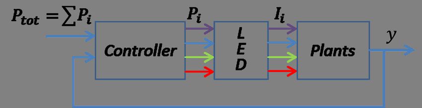
optimization of light spectrum. In order to maximize plant growth for a
given, constant illumination power, Ptot (Figure 3.1), a measure of growth
rate is needed. We have therefore studied the potential of using steady-state
chlorophyll a fluorescence at 740 nm, F740, for that purpose. The advantage is
that the fluorescence response is fast, remotely measured on canopy level and
non-destructive to the plants. Therefore, fluorescence is indeed a promising
candidate to be used as a biological feedback in a closed loop aiming at finding
optimal spectra for maximized plant growth.
The fraction of absorbed light that is used for photosynthesis, re-emitted
as heat, or re-emitted as fluorescent light will vary, for example as a function
of plant status and illumination intensity. This has been studied both on
leaf level [33] and on canopy level [34]. For example, the relative level of
fluorescence is negatively correlated with photosynthesis (i.e., desirable plant
growth) at low light intensities, while it is positively correlated at high light
intensities and under stress [35], [36]. For healthy plants exposed to light
with only small variations in intensity, a reasonable assumption is that the
photosynthetic rate and the total fluorescence are positively correlated. A
21Chapter 3 Research areas
Figure 3.1: To find an optimal spectrum, i.e., how to distribute the power Ptot
among the different diode groups by feedback control, one needs to
find a quantity of plant growth that can be measured remotely and
online. Within this thesis we investigate if steady-state chlorophyll a
fluorescence at 740 nm, F740, can be a candidate measure y. Pi is the
power to each LED group, and Ii is the corresponding intensity of the
emitted light.
strong such correlation was also found in the experiments presented in Paper A
and Paper C. Under such an assumption, the maximum photosynthetic rate
for a predefined total power, Ptot , corresponds to the spectrum that maximizes
the fluorescence, F740.
Now, assume that N different LED colors are available. Then F740 depends
on all the LED sources, i.e.,
F 740 = f (P1 , ..., Pi , ..., PN ), (3.1)
where Pi is the electrical power applied to the i:th group (color) of LEDs and
f is a scalar function. For a predefined total power Ptot we may write
N
X −1
PN = Ptot − Pi . (3.2)
i=1
As our assumed optimization goal is to maximize F740, the gradient of F740
should be zero with respect to all sources, assuming that a (global) maximum
exists. Differentiating Eq. 3.1 w.r.t. Pi , and using Eq. 3.2, give
dF 740 ∂f ∂f ∂PN
= + (3.3a)
dPi ∂Pi ∂PN ∂Pi
∂f ∂f
= − = 0 for all i. (3.3b)
∂Pi ∂PN
The last equality implies that the fluorescence gains, defined as ∂F 740/∂Pi
(i.e., ∂f /∂Pi ), should optimally be equal for all LED groups. As we are
only interested in how the fluorescence gains relate to each other, the actual
relation between growth and F740 need not be known, as long as they are
positively correlated to each other. The control task then fits to a combination
223.2 Stress detection
of extremum seeking control (see [37] and references therein) to track the
fluorescence gains, and self optimizing control [38] to aim for equal gains [39].
In principle, when not being at the optimum, the controller would increase
the power to the LEDs with the highest gain and reduce the power to the
one(s) with the lowest gain.
Accordingly, our hypothesis is that with the setup presented above, the
controller will adjust the spectrum towards the one that maximizes the short
term photosynthesis. When implementing the suggested controller, one could
include limitations on for example B:G:R:FR ratios, in order to ensure good
morphology. It should be noted though, that the optimal spectrum in the
long run might differ from the one that maximizes the photosynthesis in the
short term. For example, initially applying a spectrum that stimulates leaf
expansion, rather than photosynthesis, can lead to better light interception
and thereby higher biomass in the long run.
3.2 Stress detection
If plants are subjected to inhibitory environmentally stress, the growth ef-
ficiency is reduced. These stressors can be categorized as abiotic or biotic.
Light, drought, and salinity stress belongs to abiotic stress factors while in-
sects and pathogens, such as fungi and bacteria, belong to biotic stress factors.
If the stressors are detected at an early stage their negative impact can be
minimized by removing plants or apply early treatment. Standard methods
for stress detection are often destructive or disruptive [40], hence, not an
option for on-line detection. Different optical sensors have been investigated;
hyperspectral images, mulitcolor fluorescence images and fluorescence spectra.
However, sensor-based phenotyping is still at an early stage of development
and not yet commonly applied in field [41], [42].
We have conducted experiments in order to evaluate if the dynamics in
the fluorescence response to weak light excitations can be used as features
in a machine learning context, to evaluate if plants are stressed or not. The
fluorescence has the advantage that it can potentially react on environmental
changes prior to when the changes are visible to the human eye. Further
strengths with our method is that the measurements are done on-line, remotely
on canopy level, and that the plant neither needs to be dark adapted nor
exposed to saturating light. Instead, market available greenhouse LED lamps
are used to excite the fluorescence signal and a photodiode with a bandpass
optical filter could be applicable for the detection. With this relatively cheap
setup it could be economically justifiable to distribute sensors over a large
23Chapter 3 Research areas greenhouse. Features from the fluorescence signal that potentially could discriminate between stressed and healthy plants can be extracted in many ways. The alternative used here is to treat the excitation light as the input signal, u, and the fluorescence as the output, y, and from experimental time-series data use system identification to create a dynamic model of the system. Features could then be extracted both from the time and frequency domain. In previous work on light stress, frequency domain characteristics were shown to correlate with level of stress [43]. Here, we focus on features in the time-domain. Further on, other growth parameters could be included in a classification algorithm; such as plant age or development status, temperature, relative humidity etc. With a large set of annotated data, a classification algorithm can then potentially be tuned to diagnose whether the plants are healthy or not. 3.3 Light intensity optimization If there is a real time, non-destructive way of biologically measuring the pho- tosynthetic efficiency on canopy level at the current light intensity, one could potentially optimize the light intensity for minimized power consumption and maximized growth. Many parameters can potentially affect the optimal light illumination, such as development status of the crop, time of the day, abiotical or biotical stress factors, or other environmental factors. An infrared gas analyzer can be used to measure the instant photosynthetic rate, in terms of carbon dioxide uptake per leaf area and time. This is done by measurements of carbon dioxide, oxygen, and vapor, in a controlled air flow, throw the leaf cuvette that enclose a part of a leaf. In Figure 3.2 two examples are shown, one with an built in light source (a) and one with a clear window (b) letting the ambient light hit the leaf. Such instruments are not suitable for the feedback task, being too expensive and not aggregating over canopy illuminated by the lamp, but valuable as a reference instrument in research. We have investigated if the chlorophyll fluorescence, ChlF, can be a candi- date signal to be used for the purpose of online light intensity optimization. More specifically, the fast ChlF gain, calculated as the amplitude of the ChlF caused by (1 Hz) pulses in the incident light. Hence, the ChlF gain is used as an estimate of the derivative of the absolute ChlF w.r.t. incident light. If the plant use the light equally, independently of the intensity level, the relation between incident light and ChlF would be constant, in other words a constant derivative or gain. However, that is not the case. For high light intensities saturation occurs and the efficiency from incident light to photo- 24
3.3 Light intensity optimization

Figure 3.2: An infrared gas analyser, for measuring the photosynthetic rate in
            terms of CO2 uptake per m2 leaf area and s. Mounted with a leaf
            cuvette combined with a light source (left), and a clear leaf cuvette
            allowing the ambient light reaching the leaf (right).

synthesis decreases. This has also been detected in the ChlF, that for high
light intensities the ChlF gain decreases.
   Figure 3.3(a) shows the light response curves, i.e., photosynthetic rate for
stepwise increased light intensity, measured with an IRGA on sunflower leaves.
For high light intensities the photosynthesis saturates, and the efficiency be-
tween light illumination and growth decreases. To determine the level of
illumination that optimally balances energy cost and photosynthetic rate is
complex. However, aiming for a high photosynthetic rate, and a high effi-
ciency from incident light to photosynthesis, then the light level where the
photosynthetic rate starts to saturate is optimal.
   Figure 3.3(b) shows the normalized ChlF gain, measured with a spectrom-
eter on canopy level. These measurements were done simultaneously with the
light response curves in (a). The ChlF gains have a concave shape, and the
peak coincides with the light intensity where the light response curve starts
to saturate.
   We propose to use the ChlF gain as a feedback signal, y, in a control loop
to control the light intensity level, u, towards the point that maximizes the
objective function J(u) = y, i.e.,

                                   max J(u).                                (3.4)
                                     u

For a concave objective function, J(u), without local extrema, this can be
achieved using an extremum seeking controller.

                                                                              25
Chapter 3 Research areas
Sunflower Sunflower
35 1
30
0.8
25
20 0.6
15
0.4
(Exp S1) wc=0.4 (Exp S1) wc=0.4
10 (Exp S2) wc=2.5 (Exp S2) wc=2.5
(Exp S4) wc=7.6 0.2 (Exp S4) wc=7.6
5 (Exp S5) wc=25.4 (Exp S5) wc=25.4
(Exp S3) wc=27.7 (Exp S3) wc=27.7
0 0
100 200 300 400 500 600 700 800 100 200 300 400 500 600 700 800
(a) Sunflower, photosynthesis. (b) Sunflower, fluorescence gain.
Figure 3.3: Experiments on Sunflower. (a) Photosynthetic rate versus incident
light. (b) Normalized ChlF gain versus incident light. The filled dia-
monds indicates the light level where the ChlF gain has its maximum.
Ongoing experiments
The implementation of an extremum seeking control strategy in physical ex-
periments is ongoing. This is beyond the scope for this thesis, but we will
briefly present some of the challenges and ways towards a working solution.
The experiments presented in this section are done on lettuce.
The first challenge encountered was that the experimental ChlF gain re-
sponse behaved differently depending on light history, and more specifically,
whether the light is increasing or decreasing. The phenomenon of trajecto-
ries that depend on direction can be described by hysteresis [44] or direction
dependent dynamics [45].
Figure 3.4(a) shows the ChlF gain as a function of lamp input for two
different experiments on lettuce. In both cases the experiments started at low
intensity, stepwise increasing the intensity and then decreasing it sometime
after a maximal ChlF gain had been observed. For these experiments the
fluorescence gain was higher when the light was increasing than when it was
decreasing.
In the first set (blue stars) the intensity increased with lamp setting ∆u = 10
every ∆t = 20 sec (approximately corresponding to a rate of 13 µmol m−2 s−1 /min)
and in the second run (red circles) the step size was larger (lamp setting 100)
and was held for 10 min (hence a rate of about 4.3 µmol m−2 s−1 /min). Both
of the two settings capture a maximum at approximately the same intensity
when increasing the light, but none of them found it again when decreasing
the light.
263.3 Light intensity optimization
4200 2400
2350
4000
2300
ChlF gain, y
ChlF gain, y
3800
2250
3600
2200
3400
2150
3200 u = 10, t = 20 sec 2100
u = 100, t = 10 min u = 25, t = 5 min
3000 2050
200 400 600 800 1000 500 600 700 800 900
Lamp setting, u Lamp setting, u
(a) Manually changed lamp settings (b) Controller changed lamp settings
Figure 3.4: Experiments on lettuce. ChlF gain as a function of incident light in-
tensity. (a) Manually increased and then decreased the light intensity.
(b) A controller increased the light intensity.
If implementing the control strategy suggested in Paper E, without taking
this phenomenon into consideration, the intensity will drift towards higher
values. One example of this is presented in Figure 3.4(b), where a controller
has changed the light in steps of lamp intensity 25 (10 µmol m−2 s−1 ) every
5 minutes. The intensity starts at 500 and increases stepwise. So does also
the ChlF gain, until the intensity input is 750. Then the ChlF gain decreases
slightly for the first time and, hence, the controller changes direction and
decreases the intensity for the next step. However, when decreasing the in-
tensity, the response becomes lower compared to when moving in the positive
direction. Hence, the controller decides to increase the light intensity again.
This process is repeated such that a decrease is followed by one to three in-
creasing steps. As a consequence, this leads to a successive increase in light
intensity and an overall decrease in ChlF gain, contrary to the purpose of the
extremum seeking scheme.
Another thing that complicates the task, is that the peak in the ChlF gain
is not always very sharp, in the sense that the peak can be followed by almost
a plateau. One way of handle that is to change the objective function, J(u),
for example, by multiplication with a straight line
J(u) = y · (−k · u + m), (3.5)
where y is the ChlF gain, u is the light intensity and k and m are tunable
scalars. Figure 3.5 shows how the objective function changes when multiplying
with different lines (constant k and m for each line, highest k-value represented
in the blue line, stepwise decreasing to k = 0 for the orange line).
27Chapter 3 Research areas
This is also a way of pushing the location of the maximum in a certain
direction (black diamonds point out the maximal value for each objective
function). Tuning the line thus gives the grower means to speed up or slow
down the growth while still having an adaption to the plants state.
A new sensor is under development. The detection is done with a lock-in
amplifier, which can detect very small AC signals, i.e., the fluorescence, in the
presence of large broad spectrum noise, e.g., the reflectance in all wavelengths,
including the fluorescence region. Compared to the current setup with the
spectrometer, this setup will be must faster (kHz range instead of Hz) and
the generated excitation intensity will be even lower. The ChlF gain is now
measured as the amplitude of the light (in the 740 nm-region), at the frequency
used for the excitation lamp. Hence, we expect that we more or less measure
the same thing, i.e., the increase in fluorescence given a small excitation signal,
at the current background light.
Figure 3.6 shows the ChlF gain calculated with the spectrometer (blue line)
and the new sensor (red line) simultaneously. The light is stepwise increased
from 225 to 475 µmol m−2 s−1 (∆u = 10 µmol m−2 s−1 , ∆t = 4 min). Both
sensors detect a peak approximately at the same light intensity. However, the
new sensor detects a faster decreasing ChlF gain when passing the maximum,
which is beneficial from a control perspective. Another advantage with the
new instrument is that it is much faster than the spectrometer and, hence,
able to detect a more stable signal even in the presence of disturbances. This
opens for the possibility of using the sensor in ambient light conditions.
1.2
5200 770
1.1
Objective function
5000 760
1
ChlF gain
ChlF gain
0.9 4800 750
0.8
4600 Spectrometer 740
New sensor
0.7
200 400 600 800 1000 8 16 24 32 40 48 56 64 72 80 88 96
Lamp Intensity, U Time, min
Figure 3.5: Objective function, when Figure 3.6: ChlF gain measured with
multiplied ChlF gain with a spectrometer (blue line)
different linear functions and the new fluorescence
according to Eq. 3.5. sensor. Stepwise increase
of light intensity from 225
to 475 µmol m−2 s−1 .
28CHAPTER 4
Summary of included papers
This chapter provides a summary of the included papers.
4.1 Paper A
Linnéa Ahlman, Daniel Bånkestad, Torsten Wik
Using chlorophyll a fluorescence gains to optimize LED light spectrum
for short term photosynthesis
Computers and Electronics in Agriculture,
vol. 142, pp. 224–234, 2017.
A series of experiments were conducted on basil plants in order to examine
whether remotely sensed steady-state chlorophyll a fluorescence at 740 nm,
F740, can be used as a control parameter in a feedback loop, aiming at ad-
justing the incident light spectrum for maximal plant growth. A second goal
was to investigate if the derivatives of the chlorophyll fluorescence w.r.t. ap-
plied powers (fluorescence gains) change relative to each other for different
light intensities and spectra. Using one LED group at a time, a high cor-
relation between steady-state chlorophyll a fluorescence at 740 nm, remotely
measured at canopy level, and photosynthetic rate, PN, measured on leaf, was
found. This indicates that F740 can be used as a relative measure of PN, at
least for the spectra and (low) light intensities being investigated. For dif-
ferent operating points, having a wide variety of spectra and intensity levels,
29You can also read