Risk, Risk Aversion, and Agricultural Technology Adoption A Novel Valuation Method Based on Real Options and Inverse Stochastic Dominance
←
→
Page content transcription
If your browser does not render page correctly, please read the page content below
Q Open, 2021, 1, 1–26
https://doi.org/10.1093/qopen/qoab016
Advance access publication date: 22 July 2021
Article

Risk, Risk Aversion, and Agricultural
Technology Adoption ─ A Novel Valuation

                                                                                                                  Downloaded from https://academic.oup.com/qopen/article/1/2/qoab016/6325550 by guest on 05 December 2021
Method Based on Real Options and
Inverse Stochastic Dominance
Alisa Spiegel1 , Wolfgang Britz1 and Robert Finger                                 2,∗

1
  Institute for Food and Resource Economics, University of Bonn, Meckenheimer Allee 174, 53115
Bonn, Germany
2
  Agricultural Economics and Policy Group, ETH Zurich, Sonneggstrasse 33, 8092 Zurich, Switzerland
∗
 Corresponding author: E-mail: rofinger@ethz.ch
Received: March 20, 2021. Accepted: June 29, 2021

Abstract
Risk and risk preferences belong to the key determinants of investment-based technology adoption
in agriculture. We develop and apply a novel approach in which an inverse second order stochastic
dominance approach is integrated into a stochastic dynamic farm-level model to quantify the effect of
both risk and risk aversion on the timing and scale of agricultural technology adoption. Our illustrative
example on short rotation coppice adoption shows that risk aversion leads to technology adoption that
takes place earlier, but to a smaller extent. In contrast, higher levels of risk exposure lead to postponed
but overall larger adoption. These effects would be obscured if technology adoption is not analyzed
in a farm-scale context or considered as a now-or-never decision, the still dominant approach in the
literature.
Keywords: Risk preferences, farm-level investment decision, stochastic dynamic programming, inverse stochastic
dominance, perennial energy crop
JEL codes: Q1

1 Introduction
Decisions to take up new activities and/or adopt new technologies are of crucial relevance
for farm success (Blandford and Hill 2006, p.43; Kumar and Joshi 2014) and reflect produc-
tion, market, technological and institutional risks as inherent properties of agriculture (e.g.
Chavas 2004), as farmers are often risk averse (e.g. Iyer et al. 2020). This is confirmed in em-
pirical studies which find risk exposure, risk perception (Marra et al. 2003; Liu 2013) and
risk preferences (Liu 2013) to be among key determinants for the timing and scale of tech-
nology adoption. Thus, all three should be considered in dynamic investment analysis (Iyer
et al. 2020). Spiegel et al. (2018; 2020) demonstrated that stochastic dynamic programming
can be efficiently combined with Monte-Carlo simulations of stochastic variables followed
by a scenario tree reduction technique to study the effect of risk on timing and scale of
technology adoption in the context of a policy analysis. We extend this approach in two
directions. First, we explicitly address the risk level based on lack of knowledge and expe-
rience as a crucial determinant of technology adoption (Marra et al. 2003; Karni 2006) by

© The Author(s) 2021. Published by Oxford University Press in association with European Agricultural and
Applied Economics Publications Foundation. This is an Open Access article distributed under the terms of the
Creative Commons Attribution License (http://creativecommons.org/licenses/by/4.0/), which permits
unrestricted reuse, distribution, and reproduction in any medium, provided the original work is properly cited.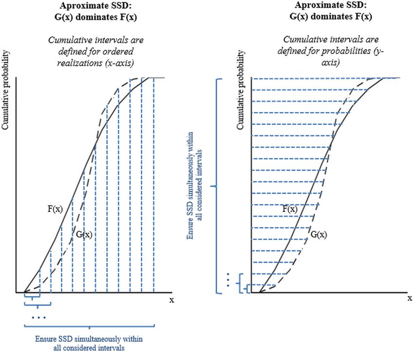
2                                                                                    Spiegel et al.

conducting sensitivity analysis. Second and more importantly, we relax the assumption of
risk neutrality underlying Spiegel et al. (2018; 2020) and hence explicitly model the effect
of risk preferences on technology adoption.
   The frequently used expected risk utility theory (Morgenstern and von Neumann 1953)
and prospect theory (Kahneman and Tversky 1979) provide a straightforward way to opera-
tionalize (perceived) risk exposure, risk perception and risk preferences to investigate effects
of both on optimal scale investment. In particular, they reveal that decision makers with a
higher risk aversion tend to adopt a new technology at smaller scales (Liu 2013; Trujillo-

                                                                                                      Downloaded from https://academic.oup.com/qopen/article/1/2/qoab016/6325550 by guest on 05 December 2021
Barrera et al. 2016; van Winsen et al. 2016). Yet, effects of risk and risk preferences on
optimal timing remain often unexplored (Meijer et al. 2015; van Winsen et al. 2016), partly
because to date there is no well-established approach to incorporate risk preferences into
dynamic investment analysis (Homem-de-Mello and Pagnoncelli 2016). The real option the-
ory provides a powerful framework to analyze optimal timing and scale of investment-based
adoption decisions at farm-level (Wossink and Gardebroek 2006; Hinrichs et al. 2008; Hill
2010; Maart-Noelck and Musshoff 2013). Furthermore, stochastic dynamic programming
is widely used for detailed analysis of managerial decisions as it reflects resource endow-
ments and can account for economies of scale. Different approaches have been proposed to
incorporate risk preferences into farm-level stochastic dynamic programming approaches
(Krokhmal et al. 2011; Homem-de-Mello and Pagnoncelli 2016). However, most of them
require a risk aversion coefficient or a risk utility function, which is difficult to determine em-
pirically (see e.g. Charness et al. 2013; Just and Just 2016; Iyer et al. 2020). Furthermore, the
computation of these approaches can become quite demanding if the programming model
comprises integers, necessary to capture indivisibilities of specific assets and economies of
scale. To cope with this, we employ the concept of second-order stochastic dominance in-
stead, namely partial ordering of alternative stochastic distributions in terms of their supe-
riority for a risk-averse decision maker. We consider this promising as it requires limited
assumptions on risk preferences and can be efficiently incorporated into stochastic dynamic
programming (Nie et al. 2012). Specifically, a set of additional constraints ensures that a
new technology or activity is only adopted at a scale (or not at all) at which it stochastically
dominates a risk benchmark given by the current farm program. There are a few exam-
ples of introducing stochastic dominance constraints into optimization models in financial
applications (El Karoui and Meziou 2006; Roman et al. 2006; Luedtke 2008; Nie et al.
2012). Although these models are concerned with the optimal shares in a portfolio of risky
assets, they are not considering resource (inequality) constraints or indivisibilities relevant
for farm-scale optimization, which implies different approaches to numerical optimization.
   We here contribute to close this gap by developing a novel farm-level stochastic dynamic
programming1 approach that quantifies the effects of risk and risk preferences on optimal
scale and timing of investment-based technology adoption. In particular, we embed the con-
cept of inverse stochastic dominance into the real options framework and demonstrate how
the proposed approach can reflect risk levels and risk preferences in an empirical exam-
ple of adopting a new investment-based activity. We call the approach DIASS—Dynamic
programming and Inverse Approximated Second-order Stochastic dominance. Using the
designed model and applying it to an empirical case study, we test for this specific case
whether risk aversion (vis-à-vis risk neutrality) leads to earlier technology adoption at a
lower scale. Moreover, we test whether higher associated risk levels ceteris paribus lead to
later technology adoption at a lower scale. We also quantify the economic relevance of these
effects. Findings underline that the DIASS approach allows to simulate farmers’ decisions
more precisely and thus to better inform policy makers about expected adoption of tar-
geted investment-based technologies, for instance, regarding contributing to environment
protection, animal welfare, or digitalization.
   Our case study features introduction of short-rotation coppice (SRC) biomass energy
production systems as an investment-based new technology2 on a typical arable farm in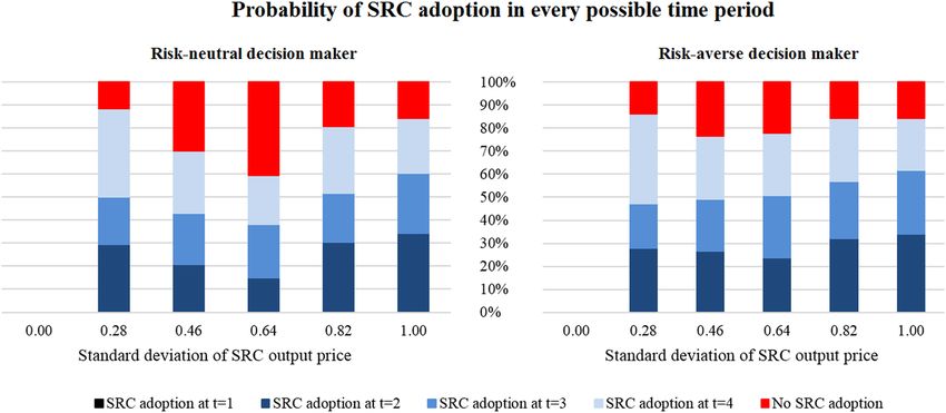
Risk, Risk Aversion, and Agricultural Technology Adoption                                       3

northern Germany. Setting up an SRC plantation with its typical production cycle of approx-
imately 20 years implies significant sunk costs for planting, coppicing and final reconversion
to arable land. Reconversion is considered as the plantation will be otherwise considered
legally as a forest, which prevents future re-conversion to arable land and claiming of farm-
ing subsidies. SRC binds land for a longer period than other currently observed land uses in
that type of farms and competes with annual crops for limited farm resources such as land
and labour. Both SRC and annual crops imply stochastic returns; the observed distribution
of returns from annual crops constitutes an observed risk benchmark. The case study thus

                                                                                                     Downloaded from https://academic.oup.com/qopen/article/1/2/qoab016/6325550 by guest on 05 December 2021
encompasses the elements mentioned above as inherent for investment-based technology
adoption in agriculture, such as sunk cost, uncertain future returns, and competition with
existing activities. It hence perfectly fits to demonstrate how the effects of risk level and
risk preferences on timing and scale of adoption can be quantified and analyzed. To this
end, we provide insights in both a generic modelling approach and in a specific case study.
The DIASS approach can be applied to any other case study by adjusting the underlying
stochastic processes and their mutual correlation, the number of investment and disinvest-
ment decisions considered, or the time horizon. We provide the code, data, all the related
documentation, as well as a graphical user interface, in Spiegel et al. (2017), in order to
facilitate use of the proposed approach for other case studies in and beyond agriculture.
   Our results show that risk aversion leads to technology adoption that takes place earlier,
but to a smaller extent. In contrast, higher levels of risk exposure lead to postponed but
overall larger adoption. These complex interdependencies between risk, risk preference and
technology adoption would be obscured if technology adoption is not analyzed in a farm-
scale context or considered as a now-or-never decision, i.e. according to the still dominant
approach in the literature.
   The remainder of this paper is structured as follows. Section 2 introduces the theoretical
background (section 2.1), develops the DIASS approach (2.2), and formulates hypotheses
(2.3). Section 3 illustrates our approach with a case study. In particular, it presents the gen-
eral layout of the designed model (3.1), the solution process (3.2), the case study character-
istics, including deterministic parameters (3.3), and the stochastic components of the model
(3.4). Our empirical results are presented in Section 4. Section 5 concludes.

2 Literature and theoretical background
2.1 State of the art of investment-based technology adoption under
    consideration of uncertainty and risk attitude
Given the production, market, institutional and technological risks involved in agricultural
production (Sunding and Zilberman 2001), plus irreversible investments and sunk costs, the
real options approach is increasingly favored over the classical Net Present Value (NPV)
approach for modelling farm-level investment decisions, including technology adoption
(Wossink and Gardebroek 2006; Hinrichs et al. 2008; Hill 2010; Kuminoff and Wossink
2010; Maart-Noelck and Musshoff 2013). The real options approach explicitly considers
the option value, or value of waiting, linked to the possibility to postpone decisions (timing
flexibility) or to adjust the investment project at a later point in time (scale flexibility), for
instance by dis-investing. It can be incorporated into a farm-level programming approach
based on stochastic dynamic programming where risk is captured by a scenario tree (Beraldi
et al. 2013; Alonso-Ayuso et al. 2014; Simoglou et al. 2014). This is usually based on bino-
mial scenario trees or lattices (Schulmerich 2010; Beraldi et al. 2013; Alonso-Ayuso et al.
2014) where model size increases quadratically or even exponentially3 with the number of
time points, which limits model complexity and timescale. These restrictions can be partly
overcome with more advanced approaches such as Monte Carlo simulation followed by
scenario tree reduction (Dempster 2006; Heitsch and Römisch 2008; Spiegel et al. 2018,
2020).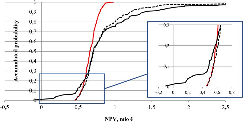
4                                                                                  Spiegel et al.

   The real options approach can be applied under different assumptions with regard to
risk preferences. Incentives to postpone a managerial decision, e.g. technology adoption,
might exist regardless of risk attitude (Dixit and Pindyck 1994, p.153). Spiegel et al. (2018)
demonstrated that in the risk-neutral context, decreasing or eliminating a risk might lead to
earlier adoption at a lower scale. However, risk preferences can influence the optimal timing
and scale of technology adoption as well (Marra et al. 2003; Liu 2013). Empirical results
highlight that European farmers tend to be risk averse (Menapace et al. 2013; Meraner
and Finger 2017; Iyer et al. 2020). That motivates the development of an approach which

                                                                                                    Downloaded from https://academic.oup.com/qopen/article/1/2/qoab016/6325550 by guest on 05 December 2021
combines the real options approach and risk aversion in a programming setting. Literature
provides no established approach for this yet (Homem-de-Mello and Pagnoncelli 2016). In
the following, we discuss the advantages and disadvantages of the dominant approaches
suggested by the literature, namely the expected utility function, using a risk-adjusted dis-
count rate, and the concept of stochastic dominance. We show that they are particularly
limited when not only optimal time and scale of technology adoption are considered, but
also competition among different farm activities for limited resources.
   Introducing and maximizing a utility function is a straightforward approach and often
used in empirical applications (Hugonnier and Morellec 2007; Shapiro 2012). Obviously,
results are sensitive to functional choice and parameterization, found as empirically chal-
lenging (Lence 2009; Crosetto and Filippin 2016). In the context of programming models,
expected mean-variance analysis initiated by Markowitz (1952) is common; it optimizes a
weighted sum of the expected mean and the variance, namely a quadratic utility function.
To avoid quadratic programming, Hazell (1971) suggested minimization of total absolute
deviations as a linear approximation of expected mean-variance analysis which is based on
absolute deviations from the mean, typically taken solely downside risk into account. These
approaches are applied frequently in programming models without state contingency where
for each time point (or in the comparative-static case, for an average one) just one combi-
nation of decision variables can be chosen. The optimization weights the outcomes from
different states based on the risk utility objective. State contingency renders calculations far
more demanding, especially if the decision variables are binaries or integers as in our case,
since the distribution of average returns per hectare of a crop depends on its endogenously
optimized state contingent acreages.
   Computational limits can be overcome by maximizing the certainty equivalent instead
and using an approximation (e.g. see Henderson and Hobson 2002). The approach re-
quires assuming a coefficient of risk aversion only, rather than formulating a risk utility
function. Meyer and Meyer (2005), Gandelman and Hernandez-Murillo (2015) and Iyer
et al. (2020) provide an overview of levels of relative risk aversion. Stable optimal behav-
ior under different levels of risk aversion requires additional assumptions about the related
risk. For instance, Černý (2004) observed a negligible effect only for small and non-skewed
associated risk. Kallberg and Ziemba (2013) found that decision makers with a ‘similar’ ab-
solute risk aversion coefficient select ‘similar’ portfolios, regardless of the utility function;
however, this result applies to normally distributed assets and a short time horizon. Fur-
thermore, the literature on risk aversion usually deals with annual volatility and employs a
distribution, rather than a stochastic process (e.g. Chavas and Shi 2015). This automatically
implies a potential natural hedging effect when accumulated over years, namely reduction
of total risk exposure due to imperfect correlation of multiple stochastic processes. Captur-
ing risk preferences by a Risk-Adjusted Discount Rate represents a conceptually different
approach, not affecting computational feasibility. In contrast to a risk-free discount rate,
a Risk-Adjusted Discount Rate reflects both the level of risk and the decision maker’s at-
titude towards this risk. Therefore, it should be adjusted as the level of risk changes over
time. More specifically, the adjustment would be specific for each farm activity, which is
characterized by a different level of risk, and at each node of the scenario tree, since the
risk decreases when approaching the leaves of the scenario tree (Brandão and Dyer 2005;
Risk, Risk Aversion, and Agricultural Technology Adoption 5
Finger 2016). Furthermore, capturing level of risk and risk aversion by one joint parameter
excludes their separate analysis.
Based on these considerations, we regard second-order stochastic dominance (SSD) as a
promising option; its application offers new insights on how risk and risk aversion affect
the timing and scale of technology adoption at farm-level. While consistent with the ex-
pected utility hypothesis (Chavas 2004), SSD only requires the underlying von Neumann-
Morgenstern utility function to be monotone and concave featuring the case of a risk averse
decision maker. Any risk-averse decision maker should therefore prefer a solution which in-
Downloaded from https://academic.oup.com/qopen/article/1/2/qoab016/6325550 by guest on 05 December 2021
corporates a new technology or activity if it is second-order stochastically dominates his
current farm program. If adoption at higher scale is riskier than the benchmark, SSD pro-
vides a lower limit on the simulated scale of adoption, while solving for the risk neutral
case should provide an upper limit (assuming that risk loving can be empirically excluded).
The opposite applies if the new technology or activity is less risky. Simulating both cases
thus allows defining the band of potential adoption scale and timing under economic ra-
tional behavior. Hardaker et al. (2004) suggests how to apply SSD to certainty equivalents
of stochastic alternatives for a given range of risk aversion coefficients. The method, called
stochastic efficiency with respect to a function is a more powerful variation of the stochastic
dominance analysis with respect to a function introduced by Meyer (1977). These methods
advance in considering a range of risk aversion coefficients simultaneously, but still require
assumptions on a risk utility function, like other alternatives described above. Additionally,
their direct implementation as constraints in a dynamic programming model with stage
consistency would be numerical quite challenging. To this end, ensuring computational fea-
sibility and measuring risk are the two most demanding issues when introducing SSD or
related concepts into a farm-level stochastic dynamic programming model. The following
sub-section discusses both and proposes solutions.
2.2 Inverse stochastic dominance and stochastic dynamic programming
According to SSD, a random variable B dominates a random variable A (i.e. B (2) A) if
the expected utility E[u(·)] of B is at least as high as that of A, (i.e. E[u(B)] ≥ E[u(A)])
(Dentcheva and Ruszczyński 2006). In general terms, the condition of SSD for a discrete
case can be formulated as follows, as long as the underlying utility function is monotone
and concave (Chavas 2004):
B (2) A ⇔ [(FA (x) − FB (x)) ∗ (x+1 − x) | x ≤ z] ≥ 0 ∀z (1)
x
where (2) stays for second-order stochastic dominance; A and B are stochastic variables
with possible realizations x; FA and FB are their cumulative distribution functions; x+1 is
the minimum possible realization higher than x.
The incorporation of SSD as a constraint into an optimization model will typically im-
ply a substantial increase in computational complexity, since it requires the introduction
of additional binary variables (Gollmer et al. 2007, 2008). Alternative (approximate) for-
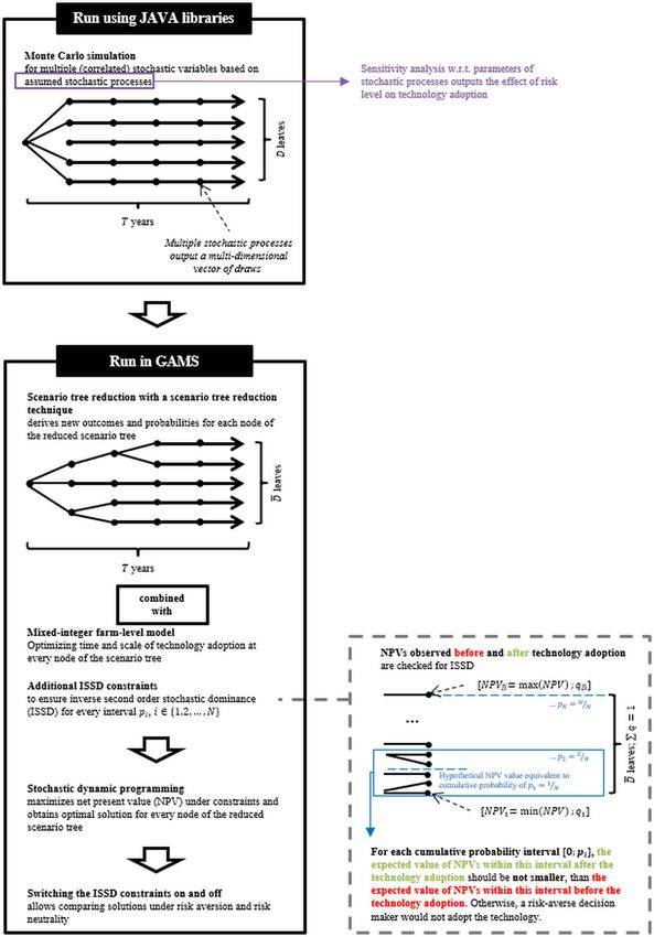
mulations of stochastic dominance are proposed to deal with this. In particular, Dentcheva
and Ruszczynski (2003) suggest a relaxation of the SSD constraint, namely defining a finite
number of compact intervals of possible realizations and ensuring SSD within all inter-
vals simultaneously. This so-called interval second order stochastic dominance approach
requires ordering realizations, which in turn depends on decision variables and leads to a
substantial increase in both the number of variables and the required solution time. This lim-
itation can be overcome if intervals are defined over the cumulative probability rather than
over realizations (Fig. 1), an approach termed inverse second order stochastic dominance
(ISSD) (Ogryczak and Ruszczynski 2002; Dentcheva and Ruszczyński 2006; Rudolf and
Ruszczyński 2008). More specifically, for a probability space (, , P) we first introduce6 Spiegel et al.
Downloaded from https://academic.oup.com/qopen/article/1/2/qoab016/6325550 by guest on 05 December 2021
Figure 1. Schematic comparison of approximate second order stochastic dominance (SSD) and inverse SSD
the following definitions (Ogryczak and Ruszczynski 2002):
F (−2) (x; p) = p ∗ E {x|x ≤ η} | p = P {x ≤ η} (2)
where F (−2) : R → R̄ is the second quantile function4 ; E{·} is the expectation operator;
x ∈ R are realizations of a random variable; and η R is the so-called target value. It is
shown that SSD of B over A is equivalent to the expected realization of B being greater
than or equal to the expected realization of B at all intervals p (Ogryczak and Ruszczynski
2002):
FB(−2) (x; p) F (−2) (x; p)
B (2) A ⇔ ≥ A
p p
⇔ EB {x|x ≤ η} ≥ EA {x|x ≤ η} ∀p = PB {x ≤ η} ∈ (0; 1] (3)
The approach does not require ordering realizations x beforehand; the target value η is
defined for each p and all x ≤ η are multiplied with the respective probabilities to define
E{x|x ≤ η} without being ordered. We first derive the distribution of returns of a farm under
the observed benchmark farm program as A representing a revealed optimal choice given the
farmer’s risk preferences. Next, we solve for B. More specifically, we determine a program
with optimal timing and scale for the new technology or activity under the condition that
it (approximately, using ISSD) stochastically second-order dominates the given benchmark
A. The original farm program A is comprised in the set of potential solutions B and might
be returned as the optimal choice. This happens if there is no stochastically dominating
solution involving the new technology or activity. Otherwise, a changed plan B is returned,
i.e. the highest expected NPV which is not riskier as the benchmark A as it dominates A
(approximately) stochastically in the second order.Risk, Risk Aversion, and Agricultural Technology Adoption 7
Specifically, we define a finite number N N of compact intervals [0; pi ] with i =
{1, 2, . . . , N} ; p1 = 1/N; and pi+1 = pi + 1/N, and ensure the condition (3) for each of
them. The narrower the intervals [0; pi ], (i.e. the higher the number N), the closer the ap-
proximation of ISSD.
Farmers’ field-, farm- and household-level decisions are driven by a wide range of fac-
tors, such as cognitive ones (perceived costs and benefits), social ones (social norms) and
dispositional ones (goals and preferences) (Dessart et al. 2019) of which we consider only
profits, risk perception and risk preferences. Assuming a farm household context without
Downloaded from https://academic.oup.com/qopen/article/1/2/qoab016/6325550 by guest on 05 December 2021
off-farm income, we take yearly profit withdrawals (net of taxes) as the objective variable,
driven by stochastic returns of the farming operations. Measuring related risk levels in each
year is challenging. Besides adjustment of the farm’s production and investment program
as endogenously optimized, yearly withdrawals can be managed by additional instruments,
such as adjustments of household expenditures or the use of short-term loans (see de Mey
et al. 2016 for holistic analysis of farm-household risk behavior). However, these instru-
ments are very difficult to observe. In addition, computational speed would be significantly
reduced if we control for ISSD at each time period and at the same time introduce additional
decision variables such as short-term loans. It is therefore relatively common to use the dis-
tribution of the NPV to assess the risk level of an investment project (Ghadim and Pannell
1999) instead of considering the annual distribution of cash inflows and outflows. This con-
cept implies that an agent only considers the distribution of his/her (discounted) terminal
wealth after the lifetime of a project. The literature suggests using a normative portfolio
characterized by a tolerable distribution (Bailey 1992; Kuosmanen 2007) if alternatives are
evaluated. In the farm context, a farmer’s observed production activities and related realiza-
tions can be considered as such a benchmark (Musshoff and Hirschauer 2007). We find it
straightforward to include the initial farming activity as the benchmark and optimize an al-
ternative one considering the adoption of a new technology, using constraints to ensure that
it stochastically dominates the status quo. Assuming that the status-quo is not based on ra-
tional behavior obscures the simulation outcome, since differences between the benchmark
and the optimal solution would not only reflect the opportunities arising from considering
the new technology, but also different behavior.
2.3 Risk analysis and hypotheses
With regard to the effect of risk aversion on the scale of new technologies, literature
indicates that higher risk aversion tend to reduce the scale (Liu 2013; Trujillo-Barrera et al.
2016; van Winsen et al. 2016). This suggests that new technologies are assessed as riskier
than those currently in use. The effect of risk aversion on timing reflects the returns if
not investing as the opportunity costs associated with the risk. Accordingly, investments
are postponed if the returns from alternative resource allocations are viewed as less risky
(Hugonnier and Morellec 2007). If opportunity costs are also stochastic and correlated with
the investment option to be exercised (as in our settings), there is a potential opportunity
for hedging and a risk averse decision maker may be more willing to exploit this by in-
vesting earlier (Henderson and Hobson 2002; Truong and Trück 2016; Chronopoulos and
Lumbreras 2017). Therefore, we hypothesize that risk aversion leads to a smaller scale and
earlier adoption (Table 1).
Previous studies often revealed differences between the ex-ante risk perception of in-
vestment projects and actual risk levels derived ex-post (Liu 2013; Menapace et al. 2013;
Bocquého et al. 2014), suggesting that investment decisions are based on subjective beliefs
(Savage 1972; Marra et al. 2003; Karni 2006). Empirical research identifies a number of
factors that affect risk perception, including age (Menapace et al. 2013), past experience
(Menapace et al. 2013), education (Liu 2013), social networks (Kassie et al. 2015), as well
as risk aversion (Menapace et al. 2013; Trujillo-Barrera et al. 2016). Perceived risk levels8 Spiegel et al.
Table 1. Formulation of the null (H0) and alternative (H1) hypotheses
Effect on
Scale of technology adoption Timing of technology adoption
Risk aversion H0: Comparing with risk H0: Comparing with risk
neutrality, risk aversion leads to neutrality, risk aversion
a lower optimal scale of accelerates technology adoption
Downloaded from https://academic.oup.com/qopen/article/1/2/qoab016/6325550 by guest on 05 December 2021
technology adoption
H1: Comparing with risk H1: Comparing with risk
neutrality, risk aversion leads to neutrality, risk aversion delays
the same or a greater optimal or does not affect the timing of
scale of technology adoption technology adoption
Factor
Higher risk H0: The higher the risk level the H0: The higher the risk level the
level lower the optimal scale of later technology adoption
technology adoption should be exercised
H1: Either risk level does not H1: Either risk level does not
influence the optimal scale of influence the optimal timing of
technology adoption or the technology adoption or the
higher the risk level the greater higher the risk level the earlier
the optimal scale of technology technology adoption should be
adoption exercised
are especially relevant in association with new technologies where lack of experience results
in uncertainty (Bougherara et al. 2017). This uncertainty might even be tagged as risk am-
biguity, or inability to formulate subjective probabilities (Barham et al. 2014; Bougherara
et al. 2017). There are hardly any studies addressing the significance of the (perceived) level
of risk for technology adoption (Meijer et al. 2015). The few existing findings are ambigu-
ous: some argue that it is one of the major determinants (Jain et al. 2015; Trujillo-Barrera
et al. 2016), while others have failed to find any significant effect (van Winsen et al. 2016).
According to the theory of real options, higher volatility, or a higher perceived risk level,
increases both the option value and the trigger price that must be reached in order to initiate
investment (Dixit and Pindyck 1994; Hugonnier and Morellec 2007). In contrast, zero per-
ceived risk would convert the problem into a classical NPV approach with no incentive to
postpone. Therefore, we hypothesize that a higher perceived risk level of a new technology
leads to a smaller scale of technology adoption and postponement (Table 1).
3 Empirical application of the DIASS approach
3.1 General layout
We develop a model based on the stochastic-dynamic programming approach where deci-
sion variables are state-contingent. We allow the farmer to introduce a new venture which
competes with established activities for (quasi-fixed) resources such as farm land and labor.
The adoption of the new activity requires investments subject to indivisibilities of assets
and returns to scale. Per unit returns from the new venture are risky and follow a stochas-
tic process, the same applies to established activities. This implies that opportunity costs
for the new activity are not known beforehand, but depend on the interaction of the level
of adoption and the states of nature. We also assume that the initial farm program before
adopting a new technology constitutes an optimal portfolio under the given stochastic re-
turns; it serves as our risk benchmark. With a set of additional constraints, we ensure that a
new venture is only adopted at a scale (or not at all) at which it second-order stochastically
dominates this benchmark. Furthermore, the decision maker has the flexibility to postpone
the adoption of the new activity, motivating the use of a real option approach. To this end,Risk, Risk Aversion, and Agricultural Technology Adoption 9
we assume that the decision about optimal time and scale of a new technology adoption is
based on an NPV maximization; subject to existing resource endowments and other farm-
level constraints; conditional to possible future developments of stochastic variables; while
ISSD constraints approximate inverse second order stochastic dominance over the endoge-
nously simulated distribution of discounted terminal wealth. The optimization problem can
then be expressed as follows:
max NPV (x; z) (4)
Downloaded from https://academic.oup.com/qopen/article/1/2/qoab016/6325550 by guest on 05 December 2021
⎧
⎪
⎪ EB {NPV (x; z)|NPV (x; z) ≤ η} ≥ EA {NPV (x; z)|NPV (x; z) ≤ η}
⎨ η: p = P {NPV (x; z) ≤ η}
i B
subject to i
⎪
⎪ pi = / N
⎩
∀i = {1, 2, . . . , N}, x C
where NPV (x; z): R → R̄ is objective function; z ∈ R are realizations of a random variable;
N N is a finite number of compact intervals [0; pi ] with i = {1, 2, . . . , N} ; and set C
represents further constraints for decision variable x, for instance, resource endowment
constraints.
Some consequences of these assumptions are worthy of closer consideration. First, we
apply ISSD to compare distributions of terminal wealth of two portfolios of risky farm ac-
tivities rather than single activities. This allows considering interaction and correlation be-
tween separate activities, including risk mitigating effects of not perfectly correlated stochas-
tic variables such as profits from different crops, i.e. a natural hedge. Second, a joint parallel
shift of resulting NPV distributions under A and B scenarios does not affect the outcome
of (I)SSD such that we can ignore levels and changes in costs and benefits independent of
the farm’s activity portfolio, for instance, fixed management costs, direct payments or other
sources of household income. This is an advantage of ISSD since such fixed costs and ben-
efits and their stochastic distribution would need to be specified if different levels of risk
aversion were considered. It reflects that ISSD is not based on the specification of a risk util-
ity function and does not require a risk-adjusted discount rate when discounting cash flows
related to investments with a differing degree of risk or to different nodes of the scenario
tree (Brandão and Dyer 2005; Finger 2016).
3.2 Solution process
The mixed-integer model is solved with stochastic dynamic programming by using a sce-
nario tree to represent uncertainty with a predetermined number of D̄ leaves. This tree stems
from first running a Monte Carlo simulation with D = 10,000 draws and subsequently
reducing the resulting tree to the desired size by applying a scenario tree reduction tech-
nique according to Heitsch and Römisch (2008).5 This allows control over overall model
size, while keeping the values assigned to each node within a certain plausible range and
hence gaining a computational advantage. Since there are multiple stochastic variables in
the model, a vector of values is assigned to each node of the scenario tree. The optimal deci-
sion with respect to technology adoption for each node of the tree is conditional to decisions
made prior to this node and the possible follow-up scenarios (Fig. 2).
The effect of risk aversion is quantified by adding the ISSD constraints to the model,
and then comparing resulting outcomes without these constraints, namely the risk-neutral
case. As mentioned, we measure risk levels based on the final distribution of NPVs and use
the currently observed behavior as the benchmark for tolerable risk. The additional ISSD
constraints ensure (approximately) that, giving due consideration to the new activity, the
distribution of NPVs under the benchmark is dominated second-order stochastically by the
final distribution of NPVs (Fig. 2).
We conduct a sensitivity analysis to capture different risk levels associated with technol-
ogy adoption by considering different parameters of the related stochastic process (Fig. 2),10 Spiegel et al.
Downloaded from https://academic.oup.com/qopen/article/1/2/qoab016/6325550 by guest on 05 December 2021
Figure 2. Schematic representation of the solution approach.
however without changing its long-term mean nor the expected mean in each year. Conse-
quently, results under a now-or-never risk neutral decision (or the classical risk neutral NPV
approach) would not change. Draws of the other stochastic processes which relate to the
activities present at the farm prior to technology adoption are obtained once and fixed.
3.3 Case study and model specification
We illustrate the DIASS approach using the example of potential introduction of a perennial
energy crop production system (SRC) on an arable farm. Setting up an SRC plantation is
an investment with high sunk costs (Lowthe-Thomas et al. 2010). Once established, the
plantation has a lifetime of approximately two decades, during which it can be coppiced
several times without being replanted. Volatile and hard to forecast prices of fossil fuels,Risk, Risk Aversion, and Agricultural Technology Adoption 11
which SRC biomass substitutes for heating purposes, imply that also future SRC biomass
prices are highly uncertain.
The combination of uncertainty, high sunk costs plus the possibility to postpone the adop-
tion decision and to adjust the scale of SRC implementation generates an option value (or
a value of postponing implementation and acquiring more information prior to making a
decision) (Pindyck 2004). SRC adoption has been analyzed using real options under risk
neutrality (Song et al. 2011; Bartolini and Viaggi 2012; Frey et al. 2013; Spiegel et al. 2018,
2020) and under risk aversion by introducing a risk-adjusted discount rate (Musshoff 2012;
Downloaded from https://academic.oup.com/qopen/article/1/2/qoab016/6325550 by guest on 05 December 2021
Wolbert-Haverkamp and Musshoff 2014). Empirical results for German farmers (Meraner
and Finger 2017) suggest risk aversion, here depicted by ISSD as a new methodological ap-
proach. Compared to previous studies, we analyze additionally the effect of different risk
levels on the timing and scale of SRC introduction by changing the risk level associated
with SRC. Equally, we compare timing and scale of SRC adoption between risk neutral and
risk-averse farmers by switching the ISSD constraints on and off.
We evaluate the option value of SRC in a farm-level context, capturing interactions with
annual crops based on competition for land and labor as fixed resources which are allo-
cated among farm activities in fractional shares. The currently observed production activ-
ities considered for the benchmark comprise the production of two types of annual crops,
one of which is more profitable, but also more labor-intensive (for instance, winter wheat
compared to rapeseed), as well as set-aside land and catch crops. The two annual crops
are characterized by gross margins following a stochastic process, while set-aside land and
catch crops are modeled with deterministic costs and introduced to fulfill the Ecological
Focus Area requirement,6 to which SRC contributes in Germany with a coefficient of 0.3
(BMEL 2015; Pe’er at al. 2016). SRC competes with annual crop production for land re-
sources, while the setting up and harvesting of SRC are usually outsourced, so that little or
no farm labor is required (Musshoff 2012). Economic considerations of introducing SRC
are thus as follows. On the one hand, SRC requires significant and irreversible investments
for establishment and final reconversion and binds land for a long time, while its price is
assumed to be stochastic. On the other hand, SRC reduces the amount of idling land or
catch crops required for the Ecological Focus Area requirement, while labor is saved due to
use of contracted services (Musshoff 2012). Consequently, labor previously used on a plot
now devoted to SRC can be reallocated to the more profitable and labor-intensive annual
crop.
In our setting, the farmer considers introducing SRC immediately or within the next three
years. He can coppice a SRC plantation every five years over a period of up to 20 years after
which it must be clear-cut, although earlier reconversion to other land uses (dis-investment)
is possible. This leads to time horizon of 24 years: a maximum of four years for possible SRC
introduction plus the 20 years of maximum plantation lifetime. Decision on SRC adoption
are based on maximizing the expected NPV, calculated from the NPV at each leaf of the
constructed scenario tree and the attached probability, conditional on risk expectations and
subject to constraints:
E [NPV ] = [q path ∗ NPVpath ]
path
T
GM(t,n),c ∗ L(t,n),c (t,n) ∗ harvQuant(t,n)
PRSRC
= q path t +
t=1 c
(1 + i) (1 + i)t
path
−iniCost(t,n) − TotalHarvCost(t,n) − reconvCost(t,n)
+ (5)
(1 + i)t12 Spiegel et al.
where (t, n) is a combination of time period and node of the scenario tree assigned to each
path; q path stands for probability of each path; path q path = 1; GM(t,n),c is gross margin of
a land use option c in time period t [euros per hectare per year, € ha–1 y–1 ]; Lt,c is fractional
land area dedicated to a land use option c in time period t [ha y–1 ]; c includes arable crop 1
(c = arable1), arable crop 2 (c = arable2), set-aside land (c = setaside), and catch crops
(c = catch); PRSRC (t, n) is biomass output price [euros per tonne of dry matter yields, € t ];
–1
–1
harvQuantt is the amount of biomass harvested [t y ]; iniCostt,p represents the actual set-up
costs [€ y–1 ]; TotalHarvCostt captures total costs on farm associated with harvest of SRC [€
Downloaded from https://academic.oup.com/qopen/article/1/2/qoab016/6325550 by guest on 05 December 2021
y–1 ]; reconvCostt,p represents actual reconversion costs [€ y–1 ]; i is an annual discount rate
[ per cent y–1 ]. The expected NPV defined in Eq. 5 is maximized subject to the following
constraints (nodes indices are left out for simplicity):
Resource endowments
āSRC,i ∗ Lt,SRC + āc,i ∗ Lt,c ≤ b̄t,i ∀i (6)
c
where āSRC,i represents input requirements for SRC [ha–1 y–1 ]; LSRC indicates the area dedi-
cated to SRC [ha y–1 ]; i represents inputs including land ( i = land) and labor (i = labor);
āc,i denotes fixed input-output coefficients [ha–1 y–1 ]; b̄t,i describes farm-level resource en-
dowments [y–1 ]; and Lt,c indicates the area dedicated to the production of each annual crop
[ha y–1 ].
Policy constraints
Lt,c = setaside + 0.3 ∗ Lt,c = catch + greenCoe fSRC ∗ Lt,SRC ≥ 0.05 ∗ b̄t,i = land (7)
where greenCoe fSRC is the ecological focus area weighting coefficient for SRC.
ISSD constraints
⎧
⎨E+SRC {x|x ≤ η} ≥ ENoSRC {x|x ≤ η} | η:pi = P+ SRC{x ≤ η}
pi = i/N (8)
⎩
∀i = {1, 2, . . . , N}, x ∈ C
where x is a set of decision variables; +SRC and NoSRC denote scenarios after and before
SRC adoption respectively; P{x ≤ η} denotes cumulative probability of η; set pi is a set of
predefined intervals of cumulated distribution.
As explained below, various relationships in the model need integer variables. Thus, in
order to avoid a mixed non-linear integer programming problem, we keep the model lin-
ear by pre-defining plots of certain sizes to be potentially converted into SRC plantation
in 5-hectare increments (i.e. providing 0, 5, 10, …, 100 ha of SRC plantation). Each plot
can be converted to SRC, coppiced, or clear-cut independently from the others, but partial
coppicing on an individual plot is not possible. Two equations linked to either a positive (0
in t-1 to 1 in t) or a negative (1 in t-1 to 0 in t) change in SRC on a plot are used to describe
set-up and reconversion costs respectively (nodes indices are left out for simplicity):
iniCostt,pl ≥ srct,pl − srct−1,pl ∗ costIni ∗ S pl (9)
reconvCostt,pl ≥ srct−1,pl − srct,pl ∗ costReconv ∗ S pl (10)
where index pl refers to a plot; costIni is a coefficient for set-up costs [€ ha–1 y–1 ]; costReconv
is a coefficient for reconversion costs [€ ha–1 y–1 ]; srct, pl is a binary variable indicating that
a plot is managed under SRC (= 1) or not (= 0) in time period t; S pl is size of plot pl [ha
y–1 ]. Maximum plantation lifetime is depicted by a year counter combined with an upper
bound (nodes indices are left out for simplicity):
aget,pl = aget−1,pl + srct,pl (11)Risk, Risk Aversion, and Agricultural Technology Adoption 13
Table 2. Input requirements and returns of alternative farm activities
Parameter Value Source
General farm characteristics
Land endowment 100 ha
Labor endowment 500 hours per year (h y–1 )
Real risk-free discount rate 3.87% y–1 Musshoff (2012)
Short rotation coppice
Downloaded from https://academic.oup.com/qopen/article/1/2/qoab016/6325550 by guest on 05 December 2021
Planting costs 2,875.00€ ha–1 Musshoff (2012)
Biomass yields every five years 68.57 t ha–1 Ali (2009)
Price of biomass yields Stochastic, see Table 3
Costs related to harvest Defined according to Eq. 13
Fixed costs 66.75€ y–1 Based on Pecenka and
Hoffmann (2012)
and Schweier and
Becker (2012)
Quasi-fixed costs 272.13€ ha–1 y–1
Variable costs 10.67€ t–1 y–1
Final clear-cut costs 1,400.00€ ha–1 Musshoff (2012)
Annual crops
Labor requirements for a more profitable crop 5.32 h ha–1 y–1 KTBL (2016)
Labor requirements for a less profitable crop 4.16 h ha–1 y–1 KTBL (2016)
Gross margins of annual crops Stochastic, see Table 3
Land uses recognized as Ecological Focus Area
Labor requirements for set-aside land 1.00 h ha–1 y–1 KTBL (2016)
Labor requirements for catch crops 0.00 h ha–1 y–1 KTBL (2016)
Gross margin of set-aside land –50.00 h ha–1 y–1 CAPRI (2017)
Gross margin of catch crops –100.00 h ha–1 y–1 de Witte and
Latacz-Lohmann
(2014, p.37)
aget,pl ≤ maxage (12)
where aget,pl is an integer variable reflecting plantation age [y]; and maxage is a constant
plantation age upper bound [y]. We also assume economies of scale related to SRC, for
instance related to transaction costs of finding a contractor or transport costs of harvest
equipment. In particular, we differentiate between fixed costs at the farm level, quasi-
fixed costs per each plot harvested and variable costs per tonne of dry matter harvested
(Pecenka and Hoffmann 2012; Schweier and Becker 2012) (nodes indices are left out for
simplicity):
TotalHarvCostt ≥ harvCostFixed + harvCostPlot ∗ S pl + harvCostYield ∗ stockt,pl ∗
p
harvestt,pl (13)
where harvCostFixed represents fixed harvest costs [€ y–1 ]; harvCostPlot represents quasi-fixed
harvest costs [€ ha–1 y–1 ]; harvCostYield represents variable costs [€ t–1 y–1 ]; stockt,pl is standing
biomass in time period t on land plot pl, [t y–1 ]; harvestt,pl indicates whether a plot is harvested
(= 1) or not (= 0).
The deterministic parameters, capturing conditions in northern Germany, are derived
from the literature (Table 2). Appendix A provides further details and also compares our
data assumptions with similar ones from the literature.14 Spiegel et al.
Table 3. Estimated parameters of stochastic processes based on historical observations
Parameter Value Source
Mean-reverting process for natural logarithm of SRC biomass price
Starting value 3.92a , ca.50 euro per
tonne of dry matter
yield (€ t–1 )
Long-term mean 3.92 Musshoff (2012)
Downloaded from https://academic.oup.com/qopen/article/1/2/qoab016/6325550 by guest on 05 December 2021
Speed of reversion 0.22 Musshoff (2012)
Standard deviation 0.28 Musshoff (2012)
Correlation coefficient with the other 0.00b
stochastic process
Mean-reverting process for natural logarithm of gross margins of annual crops
Starting value 6.02a , equal to 413 euro
per hectare (€ ha–1 )
Long-term mean 6.02 CAPRI (2017),
own
estimation
Speed of reversion 0.32 CAPRI (2017),
own
estimation
Standard deviation 0.28 CAPRI (2017),
own
estimation
Multiplicative coefficient for a more 1.05c
labor-intensive and more profitable crop
Multiplicative coefficient for a less 0.95c
labor-intensive and less profitable crop
a
Starting value are stet equal to the long term mean to exclude any possible effect of a trend
b
The assumption is based on ambiguous evidence in the literature about sign and magnitude of the correlation
(Musshoff and Hirschauer 2004; Du et al. 2011; Diekmann et al. 2014).
c
Multiplicative coefficients are assumed for draws converted back from natural logarithm into euro per hectare
3.4 Stochastic component
We assume that the natural logarithm of each stochastic variable follows a mean-reverting
process. This choice is based on the premise that the farmer is a price-taker in an envi-
ronment where market forces cause prices and gross margins to fluctuate around constant
long-term levels, for instance, under the assumption that there is no monopolistic power
(Metcalf and Hassett 1995) and/or technology is constant (Song et al. 2011). An mean-
reverting process is characterized by a long-term mean, speed of reversion and standard
deviation (Dixit and Pindyck 1994). We estimate the parameters of the process for annual
crops using data7 on gross margins of an average hectare of arable land in Germany between
1993–2012 from the CAPRI (2017) model data base following the procedure described in
Musshoff and Hirschauer (2004). Appendix B provides more details on this estimation. The
process for SRC biomass prices is based on Musshoff (2012).
The literature provides ambiguous evidence regarding the correlation coefficient between
SRC biomass price and annual crop gross margins (Musshoff and Hirschauer 2004; Du et al.
2011; Diekmann et al. 2014), while the effect of the coefficient on farmers’ behavior has
been found to be limited (Spiegel et al. 2018). This lets us assume a zero correlation between
the biomass price and annual crop gross margins, reflecting that gross margins of SRC and
annual crops are not driven by similar market and climatic influences. In contrast, we assume
that the gross margins of the two annual crops are perfectly correlated. Therefore, we use
one process for both gross margins and then adjust the draw at each node of the scenario treeRisk, Risk Aversion, and Agricultural Technology Adoption 15
Table 4. Comparison of business-as-usual scenario and introduction of short rotation coppice (SRC) under risk
neutrality and baseline risk levels
SRC introduction
Business-as-usual without an ISSD
(no SRC) constraint
Probability of introducing SRC (%)
In t = 1 - 0.00
Downloaded from https://academic.oup.com/qopen/article/1/2/qoab016/6325550 by guest on 05 December 2021
In t = 2 - 15.66
In t = 3 - 24.01
In t = 4 - 20.90
Never - 39.43
Mean area (ha y–1 ) -
SRC - 7.97
More profitable annual crop 80.16 81.36
Less profitable annual crop 17.00 8.97
Set-aside land 2.84 1.70
Catch crop 7.19 6.69
Expected net present value, (1000s €) 641.31 655.28
with multiplicative coefficients to derive gross margin levels (see Table 3). The correlation
coefficient enters stochastic processes as follows:
d prt = μSRC (θSRC − prt ) dt + σSRC dWtSRC
d gmt = μannual (θannual − gmt ) dt + ρσannual dWtSRC + 1 − ρ 2 σannual dWtannual (14)
where t is the time period; SRC indicates short rotation coppice; index annual indicates
both arable crops; prt is the natural logarithm for the price of SRC biomass; μSRC is speed
of reversion of the stochastic process for SRC biomass price; θSRC is long-term logarithmic
average price of SRC biomass; σSRC is standard deviation of logarithmic SRC biomass price;
dWtSRC is standard Brownian motion independent from dWtarable ; ρ is correlation coefficient
between two Brownian motions.
Further research might specify the alternative portfolio in greater detail, including differ-
ent correlation coefficients between gross margins of annual crops. The DIASS approach
does not imply any restrictions in this regard, but it is beyond the scope of our illustrative
purposes.
We obtain D = 10, 000 draws (see Fig. 2) from the Monte Carlo simulation. In order
to select the number of leaves in the reduced scenario tree, we performed multiple runs of
the model gradually increasing the number of leaves and noticed that the expected area
under SRC stabilizes beginning at 200 leaves (D̄ = 200 on Fig. 2). For ISSD constraints,
we consider 100 intervals8 with a 1 per cent-step (N = 100 in Fig. 2 and in Eq. 8), which
should render the impact of the approximation negligible. We performed the risk analysis
by gradually increasing the standard deviation and decreasing the speed of reversion in the
stochastic process for the SRC output price. The higher the standard deviation and the lower
the speed of reversion, the more volatile the stochastic process becomes, reaching a higher
spread and reverting to the long-term mean more slowly.
4 Results
The key results under risk neutrality and baseline risk levels are presented in Table 4. Note
that introducing SRC immediately (in t = 1) is not optimal, meaning that an option value
exists even for a risk-neutral farmer. Accordingly, the investment decision is postponed and16 Spiegel et al.
Downloaded from https://academic.oup.com/qopen/article/1/2/qoab016/6325550 by guest on 05 December 2021
Figure 3. Effect of risk preferences on the distribution of NPVs compared with the benchmark (BAU). Note:
standard deviation and speed of reversion of logarithmic SRC biomass price are 1.00 and 0.22 respectively.
exercised later, or not at all, depending on future developments. In 39.43 per cent of the
simulated cases, we find that SRC would never be introduced. The expected area under SRC
is 7.97 ha, which mainly stems from substituting the less profitable crop. This level of SRC is
not sufficient to fulfill the Ecological Focus Area requirement (16.67 ha would be required
given the total land endowment of 100 ha) and thus set-aside land and catch crops remain
in the farm portfolio (1.70 ha and 6.69 ha respectively).
As argued above, SRC requires no labor input. Thus, if SRC is introduced, a farmer real-
locates labor to the more labor-intensive and more profitable crop (compare 80.16 ha and
81.36 ha after introduction of SRC). This reallocation of resources creates an additional
incentive for adoption, which would be neglected when the technology adoption would be
analyzed as a stand-alone investment and not in the farm context. The optimization under
risk neutrality introduces SRC in some scenarios, such that the expected NPV must increase
compared to the benchmark. However, this also implies substantially higher risk as seen
in Fig. 3. The distribution of NPVs with SRC simulated under risk neutrality (i.e. without
the ISSD constraints, black solid curve) does not stochastically dominate the benchmark
(red curve): its lowest NPV realization undercuts the lowest one in the benchmark. Enforc-
ing SSD by introducing the ISSD constraints turns the NPV distribution function with SRC
in a counterclockwise direction, cutting the left-hand-side tail (black dashed curve). That
also reduces the probability of larger NPVs compared to the higher adoption rates of SRC
under the risk neutral case, underlining the tradeoff between a higher mean and a higher
risk.
We now demonstrate the effect of risk aversion and changes in risk levels on the scale of
technology adoption (i.e. the expected acreage of the farm under SRC). Fig. 4 combines the
effects of adjusting the standard deviation and mean of reversion of the stochastic process
for the SRC biomass price with and without the ISSD constraints. Our analysis shows that
risk aversion (under the ISSD constraint) does indeed lead to a smaller expected area under
SRC, which is consistent with the null hypothesis. Indeed, many white dots (risk aversion)
on Fig. 4 lie substantially below the respective black dots (risk neutrality). The ISSD con-
straints cut off the lower tail of NPV distribution as discussed above such that no SRC
adoption is observed in some leaves where it would be realized under risk neutrality. This
reduces the overall expected scale of SRC adoption. These differences can reach up to 20Risk, Risk Aversion, and Agricultural Technology Adoption 17
Downloaded from https://academic.oup.com/qopen/article/1/2/qoab016/6325550 by guest on 05 December 2021
Figure 4. Effect of increasing risk levels of short rotation coppice (SRC) biomass output prices on the
expected area under SRC.
hectares or around 50 per cent for the extreme cases, and are found to react more sensitive
to changes in the speed of reversion.
In contrast, the null hypothesis on the effect of higher risk levels on optimal scale is re-
jected in our example. Results show that even for a risk averse decision maker, a higher risk
level leads to a larger expected area under SRC. This is explained by managerial flexibil-
ity regarding the scale of investment depicted by state contingency: a farmer exploits the
opportunity of investing in a larger SRC plantation when prices are high and vice versa.
This managerial flexibility cuts off a part of the scenario tree with low SRC prices, since
SRC is only adopted if the price exceeds a certain threshold. Due to the set-up of the sensi-
tivity analysis, higher risk levels increase the spread of the scenario tree without changing
the expected mean. This not only creates a larger area where SRC is not realized and farm
income stems from the established annual crops, only, but also shifts up the expected SRC
price for the nodes where the threshold price is exceeded, which triggers a larger scale of the
investment project for these nodes. In our application, the expected mean area under SRC,
which measures the scale of adoption, increases at higher risk levels for both risk neutral
and risk-averse decision makers, even though the respective trigger price increases. For in-
stance, the expected mean area under SRC for a risk-neutral decision maker increases from
around 22 to 54 hectares when decreasing speed of reversion from 0.22 to 0.02. However,
this effect of increasing risk levels is smoothed by risk-aversion, especially when adjusting
the speed of reversion (Fig. 4).
Next, our results reveal a U-parabolic relationship between risk levels of SRC and incen-
tives for earlier SRC introduction (Fig. 5). Lower standard deviation values limit incentives
to postpone SRC introduction by reducing risk and the related option value, reflecting that
the decision problem moves towards a classical NPV analysis. A similar U-parabolic rela-
tionship can be observed between SRC risk levels and the probability that SRC will never be
adopted: there is a level of risk that implies the highest probability of never adopting SRC,
which can be quantified using our approach (for instance, in our application it is associated
with the standard deviation of around 0.64 on the left-hand side of Fig. 5). Therefore, the
null hypothesis is confirmed in our settings for lower levels of risk and rejected for greater
ones.
A comparison of the timing of SRC introduction in the case of risk neutral and risk averse
decision makers (Fig. 5) reveals that risk aversion might lead to earlier SRC introduction
(for instance, for standard deviation of 0.64 the probability of adopting in the second year
increases from 13 per cent to 22 per cent when risk aversion is considered). This is due
to the fact that risk averse decision makers exploit the hedging effect between the uncor-You can also read