SRI LANKA ECONOMIC VIABILITY OF SMALL SCALE SHRIMP (Penaeus monodon) FARMING IN THE NORTH-WESTERN PROVINCE OF
←
→
Page content transcription
If your browser does not render page correctly, please read the page content below
unuftp.is                                                                          Final Project 2014

     ECONOMIC VIABILITY OF SMALL SCALE SHRIMP (Penaeus
    monodon) FARMING IN THE NORTH-WESTERN PROVINCE OF
                         SRI LANKA

                                   Menake Gammanpila
                Inland Aquatic Resources and Aquaculture Division (IARAD)
           National Aquatic Resources Research and Development Agency (NARA)
                                  Colombo 15, Sri Lanka
                               menakegammanpila@gmail.com

                                               Supervisor:

                                            Pall Jensson
                                    Reykjavik University, Iceland
                                            pallj@ru.is

                                              ABSTRACT

Shrimp export is the second most valuable export of fish and fishery products of Sri Lanka and
it was 8% of during 2013. Among many commercial aquaculture initiatives so far, shrimp (P.
monodon) farming has been the most lucrative, but the business is subject to high risk and
uncertainties since it started in the mid-1980s. The present study evaluates the profitability and
risks associated with semi intensive small scale shrimp aquaculture practices in the north-
western province of Sri Lanka. Data and information for profitability analysis of the operation
over 10 years were collected from small scale shrimp aquaculture farms in the Puttalam district,
Sri Lanka, during April to August, 2014. Economic analysis revealed that the variable cost per
unit production and break-even production for the black-tiger shrimp through semi-intensive
culture system is 4.4 US$/kg and 2,500 kg respectively. Assuming minimum acceptable rate
of return (MARR) of this study is 15%, the NPV value at the end 10 years was found 33,003
US$ for the total capital invested and 34,993 US$ for the equity. Internal Rate of Return (IRR)
for the total capital investment is 41% and 74% for the equity. At the end of the ten years, sum
of total and net cash flow is 95,176 US$ and 84,093 US$ respectively. Pay-back period for the
capital investment is 3 years and it was two years for the equity. Sensitivity analysis indicated
that profitability was highly sensitive to changes in sales price. When the value of the sales
price falls by 20% or more, the IRR value becomes 13% and is not profitable. The sales price
has frequency of 28% of receiving negative NPV, followed by sales quantity (6%) and variable
cost (5%). Results of present study indicates that investment is highly profitable although the
shrimp farming is most sensitive to changes in sales price.

Key words: Cost-benefit analysis, Economic viability, Profitability, Shrimp farming

This paper should be cited as:
Gammanpila, M. 2015. Economic Viability of small scale shrimp (Penaeus monodon) farming in the north-
western province of Sri Lanka. United Nations University Fisheries Training Programme, Iceland [final
project].http://www.unuftp.is/static/fellows/document/menake14prf.pdf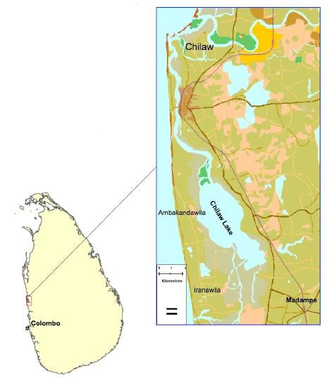
Gammanpila

                                                     TABLE OF CONTENTS

1   INTRODUCTION......................................................................................................................... 5
  1.1    Objectives .............................................................................................................................. 6
2 LITERATURE REVIEW............................................................................................................. 7
  2.1    Distribution of shrimp (Penaeus monodon) .......................................................................... 7
  2.2    Ecology and life history of P. monodon shrimp .................................................................... 7
  2.3    Present situation of world shrimp aquaculture ...................................................................... 8
  2.4    Overview of the shrimp aquaculture in Sri Lanka ................................................................. 9
    2.4.1 Importance of shrimp aquaculture in Sri Lanka ................................................................ 9
    2.4.2 Culture facility of shrimp (P. monodon) farming in Sri Lanka ....................................... 10
  2.5    The economics of shrimp farming at the farm level ............................................................ 10
3 METHODOLOGY ..................................................................................................................... 12
  3.1    Sampling site description..................................................................................................... 12
  3.2    Data collection ..................................................................................................................... 12
  3.3    Analytical technique ............................................................................................................ 13
  3.4    Profitability model of shrimp farming ................................................................................. 13
  3.5    Measures of profitability ..................................................................................................... 13
    3.5.1 Viability of investments .................................................................................................. 13
    3.5.2 Financial ratios ................................................................................................................ 15
  3.6    Risk analysis ........................................................................................................................ 15
    3.6.1 Sensitivity analysis .......................................................................................................... 16
    3.6.2 Scenario analysis ............................................................................................................. 16
    3.6.3 Monte Carlo simulation................................................................................................... 16
    3.6.4 Qualitative risk analysis .................................................................................................. 16
  3.7    Assumptions ........................................................................................................................ 16
    3.7.1 Initial investment requirement ........................................................................................ 17
    3.7.2 Total cost/Operational cost.............................................................................................. 18
    3.7.3 Production Economics of shrimp aquaculture................................................................. 19
    3.7.4 Marketing structure and gross revenue ........................................................................... 19
4 RESULTS .................................................................................................................................... 19
  4.1    Cash flows analysis ............................................................................................................. 19
  4.2    Net Present Value (NPV) in cash flow ................................................................................ 20
  4.3    Pay-back period ................................................................................................................... 20
  4.4    Internal Rate of Return (IRR) in cash flow ......................................................................... 21
  4.5    Break even point and break even price ................................................................................ 21
  4.6    Financial ratios .................................................................................................................... 21
    4.6.1 Net current ratio .............................................................................................................. 21
    4.6.2 Debt service coverage ratio ............................................................................................. 21
  4.7    Breakdown of expenses ....................................................................................................... 22
  4.8    Risk analysis ........................................................................................................................ 23
    4.8.1 Sensitivity analysis .......................................................................................................... 23
    4.8.2 Scenario summary ........................................................................................................... 24
    4.8.3 Results of Monte Carlo Simulation ................................................................................. 24
    4.8.4 Qualitative risk analysis .................................................................................................. 26
5 DISCUSSION .............................................................................................................................. 28
6 CONCLUSION AND RECOMMENDATIONS ...................................................................... 31
ACKNOWLEDGEMENTS ............................................................................................................... 35
LIST OF REFERENCES ................................................................................................................... 36
APPENDIX .......................................................................................................................................... 41

UNU Fisheries Training Programme                                                                                                                    2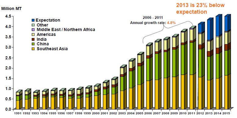
Gammanpila

LIST OF FIGURES

Figure 1: Life cycle of penaeid shrimp. ..................................................................................... 7
Figure 2: World shrimp aquaculture production by region. ...................................................... 8
Figure 3: Annual shrimp aquaculture production in Sri Lanka ................................................. 9
Figure 4: Variation of export quantity and value of shrimp in Sri Lanka .................................. 9
Figure 5: Major shrimp farming areas in Chilaw - North-western province in Sri Lanka. ..... 12
Figure 6: Total and Net cash flow of the during 10 years of operation of small scale shrimp
           farming. ................................................................................................................... 20
Figure 7: Accumulated Net Present Values and payback period of the during 10 years of
           operation of shrimp farming. ................................................................................... 20
Figure 8: IRR (Internal Rate of Return) in cash flow. ............................................................. 21
Figure 9: Financial ratios of the small scale shrimp culture in Sri Lanka. .............................. 22
Figure 10: Financial breakdown of small scale shrimp culture in Sri Lanka. ......................... 22
Figure 11: Percentages of major variable cost items in small scale shrimp farming. .............. 23
Figure 12: Impact analysis of different variable in small scale shrimp farming ..................... 23
Figure 13: Output probability distributions of Net Present Value of different variables using
            15% discount rate. .................................................................................................. 25
Figure 14: Risk analysis matrix-level of risk in shrimp aquaculture in Sri Lanka. ................. 27
Figure 15: Variations of average farm gate price/kg (>20 g) of shrimp aquaculture in Sri
            Lanka...................................................................................................................... 29
Figure 16: Production, cost and revenue of semi-intensive shrimp farming systems in Asian
            countries, 1994 ....................................................................................................... 30

UNU Fisheries Training Programme                                                                                                        3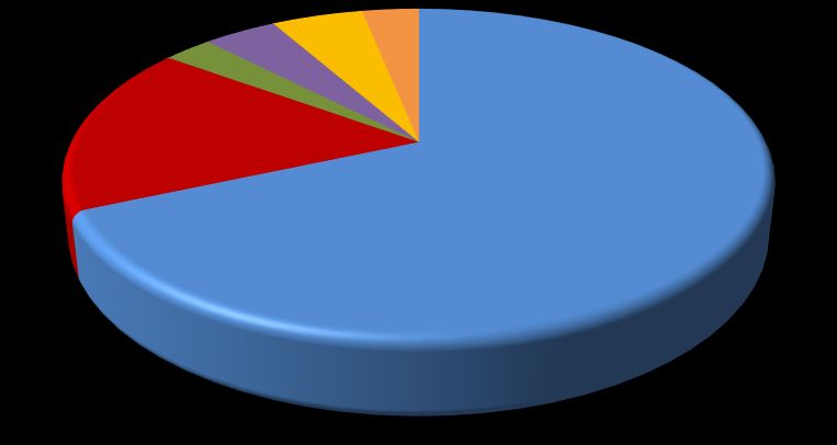
Gammanpila

LIST OF TABLES

Table 1: Comparison of past and present impacts. .................................................................. 10
Table 2: Technical/financial information and assumptions used in one farm model of small
          scale shrimp farming. ................................................................................................ 17
Table 3: Investment cost for small scale shrimp farming. ....................................................... 18
Table 4: Operational cost (fixed cost and variable cost) for one culture cycle........................ 18
Table 5: Production economic of small scale shrimp farming. ............................................... 19
Table 6: Sale price and quantities produced by one culture cycle ........................................... 19
Table 7: Different scenarios on equipment cost, quantity and sales price on NPV and IRR in
          small scale shrimp farming. ...................................................................................... 24
Table 8: Qualitative measures of likelihood and management options. .................................. 27

UNU Fisheries Training Programme                                                                                                 4
Gammanpila 1 INTRODUCTION Sri Lanka is an island state in the Indian Ocean, south-east of the Indian sub-continent between latitudes 6-10° N longitudes 80-82° E. The island is approximately 65,610 km2 with a 1,760 km long coastline. The total continental shelf area is around 30,000 km2 with an average width of approximately 25 km and extending beyond 440 km. Sri Lanka received their sovereign 200 mile Exclusive Economic Zone rights (EEZ) in 1978. The water to land ratio of 3 ha per km2 of land is considered to be one of the highest such ratio in the world (MOFE 2001). Sri Lanka has a long history of reliance on the sea and coastal areas for nutritional and economic development and well-being of the people. Today the fisheries and aquaculture sector of Sri Lanka is a major source of animal protein providing around 70% to the Sri Lankan population although the current per-capita fish and fishery products consumption level is only at 14.5 kg/year. Sri Lanka’s fisheries sector (including aquaculture) has generated 246 million US$ of revenue from the growing export market during the year 2013 and it was 2.5% of total export earnings (MFARD 2014). The shrimp industry in Sri Lanka has become one of the most important sectors of fisheries and aquaculture. Among many aquaculture initiatives so far; shrimp farming has been the most lucrative commercial aquaculture activity and a good attraction for investment over the past two or three decades. Currently shrimp export is one of major foreign exchange earner in aquaculture exports of the country earning 19.4 million US$ in 2013 (MFARD 2014). The shrimp aquaculture industry in Sri Lanka started in the early 1980s when few large multinational companies and few medium scale entrepreneurs embarked on shrimp industry (Drengstig, 2013). Although the industry initially emerged in the Batticaloa district on the east coast, the industry was subsequently established in the north-western province during the 1980s. The industry grew slowly towards the beginning of 1990 when there were a total of 60 farms covering an area of 405ha (Siriwardena 1999). As a result of an attractive package of incentives by the government the shrimp farming grew rapidly. The north-western coastal belt became the hub of the shrimp farming industry of Sri Lanka. By the end of 1999, an estimated 1,300 prawn farms covering an area of 4,500 ha and 80 hatcheries with an annual capacity of 750 million post larvae had developed in the area (FAO 2004). During this period 30-40 post larvae/m2 were stocked in earthen ponds and produced 8,000- 9,000 kg/ha/year (Drengstig 2013). The industry recorded its peak economic performances in the year 2000 by earning US$ 69.4 million worth of foreign exchange for the total exported volume of 4,855 MT. Export of farmed P. monodon accounted for almost 50% of the seafood export sector (UNEP/GPA 2003). Moreover, shrimp farming has contributed towards the development of support industries such as agricultural lime outlets/producers, fiberglass manufacturers, feed outlets, machinery supply and repair facilities, hardware stores and laboratories, cold-storage, shrimp processing, and export industry networks while providing many rural livelihoods. Shrimp farmers in Sri Lanka typically practice brackish-water monoculture of black tiger prawns (Penaeus monodon). At its blooming period, shrimp farms provided approximately 40,000 employment opportunities. However, that number dropped to approximately 8,000 after UNU Fisheries Training Programme 5
Gammanpila
disease outbreaks caused a larger number of farmers to abandon their ponds and unemployment
among smallholder shrimp farmers became a reality.
In 2010 there were approximately shrimp 603 farms operating along 120 km of coastline in the
north-western province, a dramatic decline of farming compared to 1999 (Munasinghe et al.
2010). Further, the majority (492) were identified as small scale farms, where the farmer was
actively involved in all activities of his fewer shrimp ponds. Compared to 1999, although the
farming area of during 2010 was 1,404.6 ha, no considerable difference was noted between the
production of 1999 and 2010 (3,820mt and 3,480mt respectively) (MFARD 2014).
However, smallholder farmers face uncertainty and instability, with farmers continuously
entering and leaving the industry. This is mainly because of lack of knowledge on profitable
operations and lack of understanding of the relevant inputs and of their relationships in the
entire production process (Brugère et al. 2007). Many of the studies (Philips 1992, Senarath
and Visvanathan 2001, Munasinghe et al. 2010, Westers 2012, Galappaththi and Berkes 2014)
focused more on the environmental, biological and management aspects rather than paying
critical attention to the financial aspects of the shrimp production in Sri Lanka.
Efficient financial management of aquaculture can make the difference between profits and
losses (Engle and Neira 2005). Therefore, it is essential to know the production costs and its
evolution and to determine the factors that affect farm profitability. That will help farmers to
manage their farms in a cost-effective way.
Such intervention will help to enhance confidence of small scale farmers to stick to shrimp
farming industry. Also careful investigation of the economics of shrimp farming would benefit
both producers and policymakers in designing appropriate policy measures enabling increase
of profitability in aquaculture (Ahmed et al. 2008). For this reason, need to have appropriate
information about things such as production by different culture systems, input costs and
availability, marketing demand, supply and prices making economic decisions on aquaculture
investments.
Though several researchers have looked into the biological and environmental aspects of
shrimp farming in Sri Lanka, very limited attention has been paid to the long term economic
sustainability. Therefore, the purpose of this study is to fill this gap and evaluate production
costs and the profitability (economic viability) of semi intensive small scale shrimp farms.
Further evaluating of farm-level profitability is necessary for implementation of sustainable
shrimp farming practices to convert of abandoned shrimp farms area in the North-western
province, for economic benefits for Sri Lanka.
1.1 Objectives
The purpose of the study was to:
1) Evaluate production costs in order to assess the profitability of semi intensive small
scale shrimp farms in North-western province of Sri Lanka.
2) Assess key risk factors that have significant impacts on farm profitability.
3) Provide recommendation with respect to economics to support the development of
sustainable shrimp farming practices in Sri Lanka.
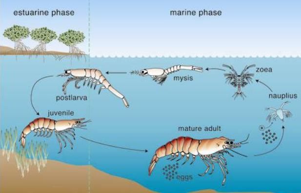
UNU Fisheries Training Programme 6Gammanpila 2 LITERATURE REVIEW 2.1 Distribution of shrimp (Penaeus monodon) Though there are more than 3,000 shrimp species worldwide, only 40 species are in fact commercially exploited (Whetsone et al. 2002). Shrimp farming is based on a few species, mainly selected from penaeidae family for their good reproductive and growth potential. The black tiger shrimp (Penaeus monodon) is the second most cultured shrimp species in the world, after whiteleg shrimp (Litopenaeus vannamei) (FAO 2010). The P. monodon is naturally distributed in Indo-Pacific, region including eastern coast of Africa and the Arabian peninsula, south-east Asia, sea of Japan and northern Australia (Holthuis 1980). 2.2 Ecology and life history of P. monodon shrimp A marine and lagoon/estuary environment are required to complete the life cycle of black tiger shrimp (Figure 1). The life cycle of penaeid shrimp is divided into 4 stages, larvae, post-larvae, juvenile and adult based on morphological, behavioral, feeding and habitat changes. The young adult shrimp migrate offshore to the ocean environment where they mature, mate and spawn. Eggs hatch after 12 - 16 hours of fertilization in nauplii larvae. The zoeae larvae, exist as plankton and feeds on microalgae and then metamorphoses in to mysis larvae after six days. The mysis larvae metamorphoses to post larvae within another three days which look like juvenile and adult. They are carried by oceanic currents to estuaries where they obtain protection and nutrition. They remain within the estuaries until they reach late juvenile/early adult stage, which is usually a period of 4-5 months. The shrimp migrate into the open ocean after becoming the early adult stage of development for the remainder of their life. In aquaculture essential environmental conditions (water salinity, temperature and other water quality parameters) are provided for each stages of shrimp life cycle. Shrimp hatcheries are produced post larvae where they are stocked in grow out facility to grown up to a marketable size. Figure 1: Life cycle of penaeid shrimp (CSIRO 2011). UNU Fisheries Training Programme 7
Gammanpila

2.3   Present situation of world shrimp aquaculture

As one of the most important seafood industries, world shrimp farming has undergone an
exponential expansion over the last few decades. In 2012, farmed crustaceans accounted for
9.7 percent (6.4 million tonnes) of food fish aquaculture production by volume but 22.4 percent
(US$30.9 billion) by value. In 2012 shrimp aquaculture accounted for 15% of the total value
of internationally traded fishery products (FAO 2014). During the first half of 2014, the volume
traded in the international shrimp market increased by 5-6% compared with the same time
period in 2013, mostly as a result of import growth to the US and east Asian markets (Globefish
2014).

High profitability and generation of foreign exchange have been a major reason in the global
expansion of shrimp culture, attracting both national and international private companies
(Primavera 1998). In the early 1980s, major improvements in hatchery production and feed
processing allowed rapid advances in shrimp farming techniques, making it possible to produce
dramatically increased yields (Shang et al. 1998). However, in 1991 its production had slowed
down due to viral disease outbreaks in major production countries.

Among the world leading shrimp producing nations, Thailand, Vietnam and Indonesia, are
ranked second, third and fourth respectively after China, the world’s largest (FAO 2014). There
are some important differences in marketing aspects among these leading shrimp-producing
nations. Shrimp production of China is mostly consumed domestically. Most of the shrimp
produced in Thailand, Vietnam and Indonesia, in contrast, is exported to major markets in the
U.S., Japan and the European Union (EU). Thailand is the world’s leading exporter of shrimp.

However, shrimp production practices today are associated with several environmental
degradation, disease out-breaks, excessive use of antibiotics and chemicals and volatility in
prices and quality (GOAL 2013). Lower production of farm shrimp in Asia and Latin America
recorded in 2012-2013 associate with the persistent disease problems, mainly white spot
disease and early mortality syndrome (EMS) (Figure 2).

Figure 2: World shrimp aquaculture production by region (1991-2015). FAO (2013) for
1991-2011; GOAL (2013) for 2012-2015. Note: M. rosenbergii is not included.

UNU Fisheries Training Programme                                                              8
Gammanpila

2.4   Overview of the shrimp aquaculture in Sri Lanka

2.4.1 Importance of shrimp aquaculture in Sri Lanka

Shrimp culture is an attractive business in Sri Lanka. It has identified one of the most successful
growth areas of aquaculture in Sri Lanka. The shrimp aquaculture is emerging as an important
source of foreign exchange in Sri Lanka. In 2013 it produced 4,430 mt and export 1,625 mt of
the value of export is 19.4 million US$ (Figures 3 & 4). The vast majority of cultured shrimp
production comes from north-western province of the country. However, out-breaks of diseases
have caused a major threat to the sustainability of the shrimp industry. The following
production figures clearly show the boom and bust nature of the industry.

                               5.000
                               4.500
                               4.000
        Production (Mt)

                               3.500
                               3.000
                               2.500
                               2.000
                               1.500
                               1.000
                                500
                                  -
                                       1990 1995 1999 2000 2001 2002 2003 2004 2005 2006 2007 2008 2009 2010 2011 2012 2013

                                                                              Year
Figure 3: Annual shrimp aquaculture production in Sri Lanka (MFARD 2014).

                               6000                                                                                           6000

                               5000                                                                                           5000
                                                                                                                                     Export value (Rs.Mn)
        Export quantity (Mt)

                               4000                                                                                           4000

                               3000                                                                                           3000

                               2000                                                                                           2000

                               1000                                                                                           1000

                                  0                                                                                           0
                                       1999 2000 2001 2002 2003 2004 2005 2006 2007 2008 2009 2010 2011 2012 2013
                                                                             Year
                                                                 Quantity (Mt)             Value (Rs.Mn)
Figure 4: Variation of export quantity and value of shrimp in Sri Lanka. Note:
including wild capture shrimp (NAQDA 2014).

UNU Fisheries Training Programme                                                                                                                        9
Gammanpila
2.4.2 Culture facility of shrimp (P. monodon) farming in Sri Lanka
The shrimp industry in Sri Lanka can be divided into following components, post-larva
production (hatchery), grow-out (shrimp farming), and shrimp processing. According to
Jayasinghe (1995) all shrimp farms in Sri Lanka are operated at semi-intensive and intensive
scale, based on major economic and technological differences. Major differences between
semi-intensive and intensive levels are in stocking density, aeration systems, farm size,
production and investment. Annual shrimp production (kg/ha) from these systems are, 6,663
for semi-intensive and 7,801 for intensive system in 1995.
A study carried out by Dahdouh-Guebas et al. (2002) before the year 2000 has categorized
three scales of production in Sri Lankan shrimp farming. Based on the classification, the
average farm area criterions for large, medium, and small-scale shrimp farms was larger than
15 hectares, between 2 and 15 hectares, and between 0.5 and 0.7 hectares, respectively. Though
during late1900s there were relatively large scale commercial operations, currently only small-
scale shrimp farms remain in the north western province area (Table 1). There are no
constructions of new farms. Munasinghe et al. (2010) reported that fifty-four percent of
farms of the Puttalam district were less than 1 hectare and 73% of farms were less than 2 ha.
Only large scale farms of > 5 ha represented 9% of farms with the remaining 18% being
between 2 and 5 ha in 2010.
Table 1: Comparison of past and present impacts (Galappaththi 2013).
Characteristics Late 90s to early 2000s Year 2012
Size of the farms Large (>10ha) /medium (2-10ha) Small scale
/small scale (Gammanpila when prices rise. Instability of market prices and income flows pose major hazards to establishing early profits and ensuring long term viability of the farm. Lack of good assessments of the industry can cause some producers to struggle to survive under fluctuating market conditions (Neiland et al. 2001). Good investment appraisal with sensitivity analysis provides a future values of the most important factors (farm gate price, feed price etc.) would allow a realistic assessment of performance of the investment under fluctuating conditions (Griffin 1995). Thus, successful management of technical and financial measures is a key factor of profitable operations (Nandlal and Pickering 2004). Production costs data help the farmers in decision making and in adjusting to changes and determining the price level under which the product cannot be sold without losses. Negative net present value (NPV) resulted when a drop in the shrimp price by 15% and the cost of production raises by 15% simultaneously in semi-intensive farming in west Bengal, east coast of India (Bhattacharya 2009). The sensitivity analysis indicates that under the uncertain scenario of international market price traditional shrimp farming system remains more economically viable than semi-intensive farming. In Philippines (Primavera 1991) finds that if the price of shrimp decreases by 20%, intensive farming, extensive farming and traditional farming fail to remain profitable with negative net present value. Only semi-intensive farming was found to be profitable in that case. Sathiadhas et al. (2009) reported the break-even point and profitability of aquaculture farming in India. The results showed that break-even price for black tiger shrimp in semi-intensive and extensive culture is worked out at US$ 3.35/kg and US$ 2.62/kg, while market sales price is US$ 7.29 to US$ 8.33/kg. The break-even price of white shrimp culture worked out to US$ 3.46/kg and US$ 1.8/kg in semi-intensive and improved extensive culture, respectively. Results of comparison study by Primavera (1993) in three management systems, extensive, semi intensive and intensive shrimp pond culture in Philippines indicates that effect of price changes on the profitability is much higher for intensive farms. Break-even price for extensive (US$ 1.83/kg), semi intensive (US$ 2.72/kg) and intensive (US$ 3.4/kg) in Indonesia suggests that the market risks of intensive farming are considerably higher. Production costs per kilogram of shrimp were highest in intensive family and commercial farms (US$ 2.7) followed by semi-intensive (US$ 2.1) and poly-culture (US$ 1.05) shrimp farming in China (Cao 2012). Intensive family and commercial farms had similar profits, the highest of all systems (around US$ 9,500 ha-1 crop-1), while semi-intensive farms obtained about half of that level of profit. This was due to high yields and better market price of intensive farming. Gonzalez-Romero et al. (2014) used a bio-economic model to define optimum pond size for commercial intensive production of the whiteleg shrimp L. vannamei. They concluded that ponds covering 2 ha are optimal based on maximum NPV (US$ 63,300), 10% interest rate and IRR (25%). Though the net present value (NPV) and the internal rate of return (IRR) of ten years farming of P. vannamei is US$ 232,000 and 15.1%, and thus very profitable, small changes in stocking density, survival rates and price can result in large losses (Sureshwaran et al. 1994). UNU Fisheries Training Programme 11
Gammanpila

Valderrama and Engle (2001) was analyzed the profitability of shrimp farming (farm size 10
to over 400 ha) in Honduras under various risk conditions. The effect of risk on profitability
was evaluated through Monte Carlo simulation. In this study feed prices and production were
correlated with other variables such as total seed costs, feed quantity, total full-time labor, total
diesel costs, debt payment, and infrastructure depreciation. Scenario analysis were defined in
order to identify possible differences in management strategies to minimize the impact of
operation failures. The results indicate that risk is more associated with low yields than high
production costs. All farms, regardless of size, need annual shrimp production of more than
450 kg/ha to avoid losses.

3     METHODOLOGY
3.1   Sampling site description

The major source of data for the study was obtained from the three small scale shrimp farms
which are located in around latitudes 7° 31' N, longitudes 79° 48' E Ambakandawila, Chilaw
within the Puttalam district in North-Western province in Sri Lanka (Figure 5).

Figure 5: Major shrimp farming areas in Chilaw - North-Western province in Sri Lanka.

3.2   Data collection

Data were collected over 20 week period from month of April to end of August 2014. Data
collection methods of the study were, a) participant observations of operating activities in farms
b) farmer interview and c) information from farm record keeping books.

For economic analysis, investment cost, production cost and return, data on yield and technical
information of farming was used for clarify production cost and assess the profitability and
feasibility of a shrimp farm investment.

Total initial investment for the present small scale shrimp farming includes cost for land,
building, fencing and equipment. Total production costs are the sum of annual fixed cost and
operational/variable cost. Variable costs are directly related to the scale of farm operations at

UNU Fisheries Training Programme                                                                  12
Gammanpila

given time period. Variable costs in production are cost of feed, post larvae, chemicals,
electricity, transport and cost for labor, etc. Fixed costs include cost for license/reports, pond
renovation, salaries of labors and consultants. Further, total production and sales price were
used to calculate gross revenue.

3.3       Analytical technique

In order to assess the profitability of the operation of a shrimp aquaculture farm over 10 years,
a model was developed by using Microsoft Excel. Data from a single farm was used as a base
case for simulation the model. The model simulates the annual activities of a farm including
production, finance, cash flow, capital replacement and depreciation, income taxes, balance
sheet and profitability measures. The model also facilitates a risk analysis. The theoretical
foundation of the profitability model and the formulas are described in the next section.

3.4       Profitability model of shrimp farming

Economic analysis can provide a systematic evaluation of aquaculture operations, which lead
to better management strategies towards economic sustainability. Economic sustainability of
any farming system is examined by its profitability based on cost and benefit analysis. Profit is
defined as the difference between the total revenue and total cost. While profit is the base for
any economic activity, economic analysis provides the basic foundation for decision making.

In aquaculture models different disciplines are used to identify important variables and their
relationships by creating formulas (Cloete 2009). A profitability model is defined as a
simulation model of an initial investment and subsequent operations. Simulation models have
been used to evaluate economic feasibility (Zuniga 2009) and optimize system design and
operations in aquaculture (Leung 1986). Profitability models can also be used as a tool for:

      •    Assessing the cost factors associated with production
      •    To assess the effects of changes in investment, operational costs in various farming
           systems and market prices on farming profitability and decision making
      •    Cost-benefit analysis of research and development options
      •    Providing an economic decision tools for researchers and stakeholders in farming.

3.5       Measures of profitability

3.5.1 Viability of investments

The profitability of investment of small scale shrimp farming will be estimated by measuring
of Net Present Value (NPV), Internal Rate of Return (IRR), Payback period (PBP) and Break-
even point (BEP) (Engle 2010; Bhattacharya 2009). The rate used to calculate the present value
is known as the discount rate (basically opportunity cost of funds plus a risk addition).

Net Present Value (NPV)

Net Present Value is used on discounted cash flows to evaluate capital investment and to give
an indication of the present value of future earnings. Essentially, net present value measures the
total amount of gains and losses a project will produce compared to the amount that could be
earned simply by saving the money in a bank or investing it in some other opportunity that
generates a return equal to the discount rate. Investments with a positive NPV would be

UNU Fisheries Training Programme                                                               13
Gammanpila
accepted; those with a negative NPV rejected, and a zero value makes the investor indifferent.
The NPV value can be calculated by using the formula below (Benninga 2008).
Where, - C0 = Initial investment, Ci = Cash flow, r = Discount rate, T= Planning horizon
Internal Rate of Return (IRR)
The discount rate at which the project has an NPV of zero is called the internal rate of return
or IRR (De Ionno 2006; Benninga 2008; Engle 2010). The IRR represents the maximum rate
of interest that could be paid on all capital invested or the discount rate at which the annual
return becomes zero, or the farm breaks even. In other words, the IRR represents the interest
rate at which capital could be borrowed for the farm, or the interest that could be earned on
capital (opportunity cost) (Siar at al. 2002).
The algorithms available in the Excel software are used for calculating NPV and IRR . These
two measures are calculated for the following cash flow series in model:
1. Total capital invested and cash flow after taxes
2. Equity and free (Net) cash flow
Payback period (PBP)
Payback period is the number of years required to recover the amount of the initial investment
from the net cash flow, resulting from the investment. In other hand it is the time required for
the cumulative NPV to become greater than zero and remain greater than zero over the rest of
the life of the project. The payback period is expressed as number of years, not as a cash amount.
It can be used to quickly identify investments with the most immediate cash returns.
Aquaculture investments are preferred with the shortest payback period (Engle 2010) other
factors being equal because of risk considerations.
Break-even point (BEP)
Break-even point is the level of production at which the total cost and total revenue are equal
(Curtis and Howard 1993), hence no profit is made and no losses are incurred. It can also be
defined as the point where the net profit is zero. The selling price, fixed costs or operating costs
will not remain constant resulting in a change in the break-even point. Hence, these should be
calculated on a regular basis to reflect changes in costs and prices and in order to maintain
profitability.
The break-even price can be compared to the cost of production of a single unit of production.
Profit is generated when break-even price is higher than the cost of production. Break-even
production and break-even price offer additional insights in to the overall feasibility of the
farming (Engle and Neira 2005).
Break-even production and breakeven selling price were calculated as follows:
Break-even production = (Fixed cost + Annuity of investment) / (Farm-gate price per unit –
UNU Fisheries Training Programme 14Gammanpila
Variable cost per unit production)
Break even sales price = Fixed cost per unit production + Variable cost per unit production
3.5.2 Financial ratios
Sustainable farming business requires effective planning and financial management. Financial
ratios are a useful management tool and key indicators of understanding of farm performance.
The most commonly used financial ratios are return on equity, return on investment, net current
ratio and debt service coverage ratio.
Net Current Ratio (NCR)
The net current ratio is a liquidity ratio. A higher current ratio indicates the higher capability
of a farm to pay back immediately its liabilities. The ratio 1.5 is mostly sufficient. The formula
used for calculating current ratio is:
Net Current Ratio: Current assets / Current liabilities
Debt service coverage (DSCR)
Debt service coverage is the ratio of cash available for debt servicing, i.e. to pay annual loan
interest and loan repayments (Engle 2010). It can be used as a useful indicator of financial
strength of the farm. Usually a debt service coverage ratio of 1.5 to 2.0 is considered as
acceptable. If below 1.0 it indicates that there is not enough cash flow to cover loan repayments
and loan interest.
Debt service coverage: (Cash flow after tax) / (Principal repayment + Interest payments)
3.6 Risk analysis
Risk analysis typically seeks to answer four questions:
• What can go wrong?
• How likely is it to go wrong?
• What would be the consequences of its going wrong?
• What can be done to reduce either the likelihood or the consequences of its going
wrong? (Arthur et al. 2004).
All businesses operate in environments loaded with risk. These include environmental,
biological, operational, financial and social risks. Therefore, it is important to evaluate the risks
associated with a business before investing in it (Cloete 2009). In Sri Lanka shrimp aquaculture
is considered a high risk business, as it involves relatively high operational cost and uncertainty
of shrimp survival during the culture period. Risk is associated with the natural variation in
factors affecting profitability over time (Okechi 2004).
Risk analysis provides measures of uncertainty with respect to changes in input variables, such
as variable and fixed cost, initial investment cost, production, sales price and interest rates.
Therefore, it is significant to identify risk early on in the farming and develop an appropriate
risk response plan. There are mainly three techniques used for assessing risks of investments:
UNU Fisheries Training Programme 15Gammanpila Sensitivity Analysis, Scenario Analysis and Monte Carlo Simulations (Brigham and Houston 2004). 3.6.1 Sensitivity analysis Sensitivity analysis is used to see the effect of changes in one input variable (for example fixed cost, variable cost, equipment cost, production quantity or sales price,) at a time on the profitability of the production. It also identifies the areas where an improvement in performance may have a positive impact on economic performance (Losordo and Westerman 1994). 3.6.2 Scenario analysis The scenario analysis evaluates the impact of changes in input of more than one variable at the same time looking at for example the optimistic, pessimistic and very pessimistic conditions. 3.6.3 Monte Carlo simulation Monte Carlo simulation is the most advanced tool for risk assessment. Monte Carlo simulation techniques were used to generate values for individual cost and quantity parameters based on the probability distributions. It is used to specify a probability distribution of the outcome as a function of each of the uncertain input factors. The risk is then the probability of a negative outcome (negative NPV). 3.6.4 Qualitative risk analysis The qualitative risk analysis was used to assessment of the impact of the identified risk factors. The risk matrix ranks probability of risk depending on the impact they could occur and in case of risk occurring of non-numerical ranges such as low, moderate, high and extreme high. Probability of occurrence and impact level of a risk matrix was developed in order to better understand the risk exposure. These include of environmental risks (e.g. severe weather events, poor water quality), biological risks (disease, lower growth rates, seed quality, predation etc.), operational risks (equipment failure, sharing of equipment, use of chemicals and supplementary feed), financial risks (e.g. sales price changes, currency fluctuations, escalating taxes and interest rates, decreasing market demand, access to credit, increasing production cost) and social risks (lack of skilled manpower, pouching, competition from other sectors). Information for analysis were gathered from reports, case studies, news articles, published research, onsite/field visit and farmers themselves. 3.7 Assumptions For economic analysis, data on yield, cost and return of farming used for clarify production cost, assess the profitability and feasibility of an investment. Total production costs included the sum of annual fixed cost and operational/variable cost. Variable costs are directly related to the scale of farm operations at given time period. Variable costs in production are cost of feed, post larvae, chemicals, transport and cost for labor, etc. The costs and benefits were calculated on per farm basis (6,500 m2) and all the inputs and output related to current study are based on price at the 2014 and US dollars (US$) exchange rate is 130 Rs/US$. The financing of the small scale shrimp farm was assumed to be 40% equity and a loan of 60% of the total investment required, at 11% interest rate, charge and management UNU Fisheries Training Programme 16
Gammanpila

fee for loans is set at 2% and loan to be paid back over 10 years. Depreciation was calculated
using the straight-line method (equal depreciation costs per annum over the asset’s life).
Depreciation on buildings was assumed to be 4% each year, equipment by 10% and other
investment by 20%. The average accounts receivable from debtors were assumed to be 20% of
revenue and accounts payable for creditors were assumed to be 15% of variable costs.
Dividends to shareholders are expected to be 10% of profit after income tax which is 8%. We
assumed a 15% of discount rate for study (Table 2). Culture period is 4 months and usually two
culture cycles were operated during the year.

Table 2: Technical/financial information and assumptions used in one farm model of
small scale shrimp farming.

                                                Value
Technical Information
Land area (ha)                                  1.0
Culture pond area (m2)                          6,500
Average pond depth (m)                          1.0
FCR                                             1.3
Stocking Density (PL/m2)                        21
Survival Rate (%)                               63
Culture period (months)                         4
Culture cycles/year                             2
Initial weight of fingerling stocked (g)        0.01
Initial number of fingerling                    140,000
Final harvest weight of individual shrimp (g)   27
Financial information
Loan                                            60%
Equity                                          40%
Loan interest                                   11%
Loan repayments                                 10 years
Loan Management fees                             2%
Assumptions
Dividend                                        10%*
Debtors (account received)                      20%*
Creditors (Account payable)                     15%*
Depreciation of buildings                        4%*
Depreciation of equipment                       10%*
Depreciation of others                          20%*
Discounting rate                                15%*
Income tax                                       8%
Planning horizon (years)                          10
*Assumed by author
Exchange rate: 1 US$ = 130 Rs.

3.7.1 Initial investment requirement

Shrimp aquaculture businesses require high levels of capital investment. Total initial
investment for the present small scale shrimp farming was 27,000 US$ (farm log book). Of the
total, 17,700 US$ was for purchasing land (1 ha), including already constructed earthen ponds,
because the entire analysis is based on the utilization of an abandoned shrimp farm. There were
three ponds extent in one ha of land area, two ponds were used for farming and other was used
as sedimentation/stock pond. Other investments were 1,600 US$ for permanent building, 3,350
US$ for fencing and 4,350 US$ for equipment (Table 3). The total capital requirement for
initial operation is somewhat higher than total investment and the difference is called working

UNU Fisheries Training Programme                                                            17
Gammanpila
capital. It is the amount of money that necessary to operating the farm until the first sales of
shrimp. The total working capital value for present study was US$ 1,000 (Appendix 2).
Table 3: Investment cost for small scale shrimp farming.
Investment Cost (US$)
Total Cost (US$)
Investment for land + ponds 17,700
Buildings 1,600
Fencing 3,350
Cost of equipment
Refrigerator 465
Generator 921
Water pump 500
Paddle wheel 2,464
Total 27,000
3.7.2 Total cost/Operational cost
Operating costs are the expenses which are related to the operation of a farm, including fixed
cost and variable cost (Table 4). The variable cost for the single culture cycle of operation was
US$ 10,264 for production of 2,350 kg per culture cycle or US$ 4.37 per/kg of shrimp. There
were two culture cycles per year, so variable cost per year is estimated as US$ 20,528 and total
production per year was 4,700 kg. Fixed cost is estimated at US$ 2,536 per single culture cycle
and US$ 5,012 per year. The total cost of operations for one year period is valued at US$ 25,540.
Table 4: Operational cost (fixed cost and variable cost) for one culture cycle
Total/Operational cost (US$) for one culture cycle
Number of units Unit cost (US$) Total cost(US$)
Fixed Cost
License/reports (Year) 3 20 60
Labor charges (2×4 months) 8 155 1,240
Consultant fees (per month) 4 154 616
Pond renovation 2 310 620
Total Fixed Cost 2,536
Variable Cost
Post Larvae 140,000 0.01 969
Feed:
Commercial feed 2,850 1.73 4,931
Supplementary feed 480 1.4 672
Electricity 9,150 0.12 1,102
Chemicals
Lime 4000 0.08 338.46
Dolomite 7000 0.19 1346.15
Other 315.39
Transport cost (fingerlings) 40
Fuel 200
Harvesting charges 300
Other (telephone, etc…) 50
Total Variable Cost 10,264
TOTAL COST 12,800
UNU Fisheries Training Programme 18Gammanpila
3.7.3 Production Economics of shrimp aquaculture
Total production for the 6,500 m2 water area was 2,350 kg of shrimp after one production cycle
which is 4 month of culture period (Table 5). There are two production cycles per year, total
annual shrimp production at this rate was 4,700 kg or 7,230 kg/ha/year. The stocking density
is 21 post-larvae per m2, average survival rate was 63 percent, while initial average weight of
post larvae 0.01 g and end of the culture cycle, average size of the harvested shrimp was around
27.0 g. Feed conversation ratio (FCR) was 1.3.
Table 5: Production economic of small scale shrimp farming.
Month Average weight (g) Number of shrimp Total weight (kg) Survival rate (%)
0 0.01 140,000 1.4 100
1 4.5 112,000 504 80
2 13.6 98,000 1,333 70
3 19 90,000 1,710 64
4 26.6 88,200 2,350 63
3.7.4 Marketing structure and gross revenue
The range of sales price for the marketing varies with size of shrimps being produced by the
farm. There are also differences in the markets supplied, domestic versus export. The gross
revenue for one culture cycle was calculated by multiplying the total amount of production
(2,350 kg) by its sales price (US$ 8.31) (Table 6). Gross revenue of net profit was calculated
as the difference between gross revenue from shrimp sale and total cost of production including
fixed cost and variable costs, depreciation, taxes, etc.).
Table 6: Sale price and quantities produced by one culture cycle
Number of units (kg) Sales price (US$) Gross revenue (US$)
Total production 2,350 8.31 19,528
4 RESULTS
4.1 Cash flows analysis
Figure 6 shows the total and net cash flow during ten year period of small scale shrimp farming.
Because of the high initial investment cost, both total and net cash flow are negative during the
first year of study. Nevertheless, in the remaining years, both total and net cash flow are
positive and continues on trend throughout the ten years planning horizon. In 2014, equity
value in the cash flow series is US$ 11,200, which is 40% of total financing in shrimp farm
operation. At the end of the ten years, the sum over the 10 years of the total and net cash flow
is US$ 95,176 and US$ 84,093 respectively (Appendix 8).
UNU Fisheries Training Programme 19Gammanpila
15.000
10.000
5.000
0
2014 2015 2016 2017 2018 2019 2020 2021 2022 2023 2024
-5.000
US$
-10.000 Year
-15.000
-20.000 Total Cash Flow & Capital
Net Cash Flow & Equity
-25.000
-30.000
Figure 6: Total and Net cash flow of the during 10 years of operation of small scale shrimp
farming.
4.2 Net Present Value (NPV) in cash flow
The assessment of economic viability is done by calculating the viability measures like Net
Present Value (NPV) and Internal Rate of Return (IRR). Assuming that the discounting rate
(MARR) of this study is 15%, the Net Present Value (NPV) at the end 10 years was found to
be US$ 33,003 for the total capital invested and US$ 34,993 for the equity. Based on Figure 7
it was observed that the first three years the accumulated NPV of total cash flow is negative.
4.3 Pay-back period
According to the Figure 7, the pay-back period for total capital investment is 3 years. It means
that this venture needs three years to recover the original investment. The higher NPV value
and relatively short pay-back period in present study indicates that investment is highly
profitable.
40.000
30.000
20.000
10.000
US$
0
2014 2015 2016 2017 2018 2019 2020 2021 2022 2023 2024
10.000
Year
20.000
30.000
40.000
NPV Total Cash Flow 15% NPV Net Cash Flow 15%
Figure 7: Accumulated Net Present Values and payback period of the during 10 years of
operation of shrimp farming.
UNU Fisheries Training Programme 20Gammanpila
4.4 Internal Rate of Return (IRR) in cash flow
Internal Rate of Return for the total capital investment is 41% and 74% for the equity in the
present study. The IRR is higher than the 15% MARR for present study, indicating that
investment is attractive and profitable (Figure 8).
80%
70%
60%
Percentage
50%
40%
30%
20%
10%
0%
2014 2015 2016 2017 2018 2019 2020 2021 2022 2023 2024
Year
IRR Total Cash Flow IRR Net Cash Flow
Figure 8: IRR (Internal Rate of Return) in cash flow.
4.5 Break even point and break even price
Variable cost per unit production is US$ 4.37/kg and annuity of the investment is US$
4,754/year. Based on annual fixed cost (US$ 5,012) the break-even production and breack-
even price for the black tiger shrimp in semi intensive system is 2,479 kg per year and US$
6.45 respectively.
4.6 Financial ratios
In following includes the results of financial rations based on calculation of the initial setup
values.
4.6.1 Net current ratio
Net current ratio is above one which indicates that current assets are greater than current
liabilities. At the beginning of the farming the assets values are 2.4 times the liabilities values,
at the end of the ten year it was 13.6 times the liabilities values. It indicates the higher capability
of a farm to pay back immediate its liabilities (Figure 9).
4.6.2 Debt service coverage ratio
A debit service coverage ratio of greater than one indicates that farm has enough cash to pay
interest and repayments loans. (Figure 9). In the first year it was 4.7 and end of the ten year 6.1
value indicates that high financial strength of the farm.
UNU Fisheries Training Programme 21Gammanpila
16
14 Net Current Ratio: (Current
asset/Current liability)
12 Debt Service Coverage: (Cash flow
10 after tax/Interest-LMF+repayment)
Accepatable Minimum
Ratio
8
6
4
2
0
2014 2015 2016 2017 2018 2019 2020 2021 2022 2023 2024
Year
Figure 9: Financial ratios of the small scale shrimp culture in Sri Lanka.
4.7 Breakdown of expenses
Breakdown of expenses show that out of the total operational cost nearly 68% of expenses are
variable cost followed by fixed cost which are 17% of total cost (Figure 10). Feed cost represent
55% or more than a half of the variable costs, and it was 44% of total operational cost. Feed
cost must be considered as most important items for the variable cost in semi-intensive systems
followed by 19% and 11% of chemicals and electricity cost respectively (Figure 11).
Fixed cost for year - round shrimp farming was US$ 5,012 of which management cost including
labor salaries constitutes about 49% and 25% of consultant fees. License fees, renovation of
pond and canal digging contributed about another 26% of total cost.
Repayments
Financial Costs 5% Paid Divident
4%
3%
Paid Taxes
3%
Fixed Cost
17%
Variable Costs
68%
Figure 10: Financial breakdown of small scale shrimp culture in Sri Lanka.
UNU Fisheries Training Programme 22Gammanpila
Other
Harvesting charges
Fuel
Expenses
Transport cost
Chemicals/Lime/Dolamite
Electricity
Feed:
Post Larvae
0 10 20 30 40 50 60
Percentage
Figure 11: Percentages of major variable cost items in small scale shrimp farming.
4.8 Risk analysis
In shrimp farming, higher intensity is accumulated with the higher financial risk. In more
intensive systems, the probability of loss are likely to be higher. World Bank (2000) reported
that financial risk in shrimp farming comes from four sources. They are input factors
(availability of brood stock, price of post larvae, water quality, credit, etc.); output factors (sales
price, production supply to the market, etc.); design factors (site selection, etc.) and natural
factors (disease, floods, typhoons, etc.).
4.8.1 Sensitivity analysis
Sensitivity analysis was done for major investment costs including cost of equipment, fixed
and variable cost and further sales quantity and sales price. The results of the impact analysis
showed that the profitability of the small scale shrimp farm production is most sensitive to
variations in the sales price. When the value of the sales price falls by 20% or more, negative
NPV in cash flow is no longer profitable and it might destroy the economic viability of the
shrimp farm (Figure12). Though variation in the cost of equipment and operational cost (fixed
and variable) did not have a significant impact on the farm profitability, variation in variable
cost had more impact on the NPV of equity than cost of equipment and fixed costs (Appendix
9).
140.000
120.000
100.000
80.000
NPV for Equity
60.000
40.000
20.000
0
-50% -40% -30% -20% -10%
-20.000 0% 10% 20% 30% 40% 50%
-40.000
-60.000
-80.000
Deviations
Equipment Sales Quantity Sales Price
Variable cost Fixed cost
Figure 12: Impact analysis of different variable in small scale shrimp farming.
UNU Fisheries Training Programme 23You can also read