The Subprime Lending Crisis - The Economic Impact on Wealth, Property Values and Tax Revenues, and How We Got Here
←
→
Page content transcription
If your browser does not render page correctly, please read the page content below
The Subprime Lending Crisis
 The Economic Impact on Wealth, Property
               Values and Tax Revenues,
                   and How We Got Here

  Report and Recommendations by the Majority Staff
                  of the Joint Economic Committee

             Senator Charles E. Schumer, Chairman
               Rep. Carolyn B. Maloney, Vice Chair

                                     October 2007
JOINT ECONOMIC COMMITTEE OCTOBER 2007
Executive Summary
As the losses caused by the subprime lending crisis continue to work their way through the
financial markets, there is a growing awareness among policymakers and financial market
regulators that we need to prevent the continuing foreclosure wave from affecting the broader
economy. A significant increase in lax (and often predatory) subprime lending during a pe-
riod of rapid housing price appreciation put risky adjustable rate mortgages in the hands of
vulnerable borrowers who are now facing substantial payment shocks and risk foreclosure
when their loans reset this year and next.
Part I of this report shows that unless action is taken, subprime foreclosure rates are likely to
increase as housing prices flatten or decline, and the effects of the subprime crisis are likely to
extend beyond the housing market to the broader economy. The decline in housing wealth
will negatively affect consumer spending, and the forced sale of large numbers of homes is
likely to negatively impact the prices of other homes.
Part II of this report shows that, unless action is taken, the number and cost of subprime fore-
closures will rise significantly. For the period beginning in the first quarter of 2007 and
extending through the final quarter of 2009, if housing prices continue to decline, we es-
timate that subprime foreclosures alone will total approximately 2 million.
Part II also includes forward looking, state-level estimates of subprime foreclosures and asso-
ciated property losses and property tax losses, covering the second half of 2007 through the
end of 2009. For that shorter period, and assuming only moderate housing price declines, we
estimate that:
• Approximately $71 billion in housing wealth will be directly destroyed through the
process of foreclosures.
• More than $32 billion in housing wealth will be indirectly destroyed by the spillover
effect of foreclosures, which reduce the value of neighboring properties.
• States and local governments will lose more than $917 million in property tax reve-
nue as a result of the destruction of housing wealth caused by subprime foreclosures.
Part III of the report highlights the underlying causes of the subprime crisis and explains how
incentive structures in the subprime market work against the interests of borrowers and have
had much to do with the dimensions of this crisis.
Finally, in Part IV, policy options aimed at reducing foreclosures and preventing the crisis
from reoccurring in the future are offered.
1JOINT ECONOMIC COMMITTEE OCTOBER 2007
Part I: The Housing Downturn and Its Impact on
Subprime Mortgage Foreclosures
Over the past few months, as residential investment and housing prices have declined, delin-
quency and foreclosure rates for subprime mortgages have spiked sharply upward. The dete-
riorating performance of subprime loans is not suprising. As the subprime market expanded
rapidly after 2001, so did the share of adjustable rate, “hybrid” loans issued to financially vul-
nerable borrowers. The ability of these borrowers to sustain hybrid mortgages has de-
pended heavily on house price appreciation. As housing prices have flattened and de-
clined, the ability of these households to refinance their mortgages has been reduced. The re-
sulting rise in subprime foreclosures is likely to harm an already weak housing market, and
the reduction in housing wealth has the capacity to reduce consumer spending and economic
growth.
HOUSING PRICE DECLINES WILL WORSEN SUBPRIME LOAN
DELINQUENCIES AND HOME FORECLOSURES
The root of the subprime mortgage crisis is the prevalence of troubling loans called “2/28”
and “3/27” hybrid adjustable rate mortgages (ARMs) that were largely sold to financially vul-
nerable borrowers without consideration for their ability to afford them. A typical “2/28” hy-
brid ARM has a fixed interest rate during the initial two year period. After two years, the rate
is reset every six months based on an interest rate benchmark (such as the London Interbank
Bid Offered Rate, or “LIBOR”). In the current environment, resets have caused payments
to rise by at least 30 percent, to an amount that many borrowers can no longer afford.
As a result, the delinquency and foreclosure rates for subprime adjustable rate mortgages have
been sharply rising. For more information about the characteristics of subprime loans and bor-
rowers, see Box A.
When housing prices were rising, subprime borrowers could sell or refinance their homes to
pay off their loans before they reset to unaffordable rates. As housing prices flatten or de-
cline, these options dwindle. This section explains how the weakening housing market is
likely to impact subprime delinquencies and foreclosures in the months ahead. For a detailed
examination of the subprime market and its expansion, see Box B.
Subprime Lending Has Depended on Rapid House Price Appreciation
The period of rapid housing price appreciation that began in 1997 has helped fuel increased
volumes of subprime lending and masked the weaknesses in underwriting quality and preda-
tory tactics that accompanied it.
Beginning in 1997, the U.S. witnessed house price appreciation that was highly unusual in
historical terms. Between 1997 and 2006, real home prices increased by nearly 85 percent.1
Sustained price increases near this magnitude have only been observed once during the twen-
tieth century, in the period immediately after World War II2 (See Figure 1). In fact, during
2OCTOBER 2007 JOINT ECONOMIC COMMITTEE
Figure 1: U.S. Housing Market in Historical Perspective
Shiller U.S. Real Housing Price Index and Other Economic Indicators, 1938-2007
250 1000
900
200 800
700
Population in Millions
Home Prices
150 600
Percent
500
100 400
Building Costs
300
50 Interest Rates 200
Population 100
0 0
1938 1949 1960 1971 1982 1993 2004
Source: Irrational Exuberance, 2nd Edition, 2005, by Robert J. Shiller, Figure 2.1 as updated by author.
the period 2001 through 2005, the annual rate of house price appreciation accelerated. The
S&P/Case-Shiller® Home Price Index shows annual price appreciation rising from slightly
over eight and one-half percent in 2001 to more than 15 percent in 2005.
Not every part of the housing market witnessed this rate of home price appreciation. In some
states and cities there was significant price appreciation, while it was more moderate in oth-
ers. For example, Figure 2 shows the difference between home price appreciation in Michi-
gan, Ohio, California, and Florida. But price increases were sufficiently widespread to pro-
duce significant nationwide increases in housing prices.
Housing Price Appreciation Reduced Subprime Delinquencies and
Foreclosures
The deterioration in underwriting standards in the subprime market as the market expanded is
well documented. (For a discussion on declining underwriting standards in subprime lending,
see Box B.) Although underwriting standards in the subprime lending market began to de-
cline after 2001, the effects of this decline were, until recently, mitigated by house price ap-
preciation. If a borrower is struggling to make mortgage payments, but the value of his house
has appreciated, he can solve his financial problems at least temporarily by refinancing the
mortgage. Cash can be withdrawn from the increased equity in the house, and the new, higher
mortgage can be sustained for a while. The house can also be sold, and the loan principal re-
paid. However, when house price appreciation does not create equity, borrowers’ finan-
cial weakness cannot be disguised and default rates rise.
3JOINT ECONOMIC COMMITTEE OCTOBER 2007
Figure 2: House Price Appreciation Has Varied Across States
House Price Index for Homes in Michigan, Ohio, California and Florida, Q1:1995-Q2:2007
700
California
600
Florida
500
Percent
400 Michigan
300
200
Ohio
100
1995 1997 1999 2001 2003 2005 2007
Source: Office of Federal Housing Enterprise Oversight
There is systematic evidence that when home prices appreciate, subprime mortgage defaults
decline. Using a very large sample of subprime mortgages securitized between 1999 and
2002, researchers at the Center for Responsible Lending found statistically significant correla-
tions between the odds of foreclosure and cumulative price appreciation in a Metropolitan
Statistical Area (MSA).3
The option to sell or refinance also should reduce delinquencies, which are the precursors to
default and foreclosure. Recent work by economists at the Federal Reserve Bank of San
Francisco shows strong negative correlations between delinquency rates and cumulative
house price appreciation across MSA’s during 2006.4 This research also indicates that house
price appreciation significantly improved the performance of subprime loans.
SUBPRIME PROBLEMS ARE LIKELY TO ACCELERATE HOUSE PRICE
DECLINES
The Housing Market Is Contracting
Unfortunately, conditions in the housing market indicate that house price appreciation
will no longer be able to disguise the financial precariousness of the millions of borrow-
ers whose subprime adjustable rate mortgages are about to reset. The decade of steady
house price appreciation appears to be at an end. Nationally, house prices began to decline in
2006 and are now down approximately 3.2 percent from their peak in the second quarter of
2006.5
4OCTOBER 2007 JOINT ECONOMIC COMMITTEE
Figure 3: Home Production Has Outpaced Demand
600 12
New Homes for
Sale
500 10
Homes for Sale (in thousands)
400 8
Months of Supply
300 6
200 4
100 Months Supply of
2
New Homes
0 0
1980 1984 1989 1993 1998 2002 2007
Source: Bureau of the Census, U.S. Department of Commerce.
In fact, the housing market has contracted significantly for more than a year. Inventories of
unsold new homes have increased, and the monthly supply of new homes has risen (See Fig-
ure 3). The Federal Reserve has estimated that so far, declines in residential investment
have reduced the annual rate of GDP growth by about three-fourths of a percent over
the past year and a half.6
A Housing Asset Bubble May Be Bursting
As residential investment in construction declines and house prices fall, there is reason to be
concerned about the longer term prospects for housing values. There is apprehension that the
economy is experiencing the bursting of a housing price “bubble” – a situation in which hous-
ing prices are high only because market participants believe that prices will be high tomorrow.
In other words, home prices deviate significantly from the equilibrium level consistent with
market fundamentals. When an asset bubble bursts, large price appreciation can be followed
by sudden and large price declines.
If a housing price bubble does exist, then house price levels can be affected dramatically by
shifts in expectations.7 There is some evidence that expectations about housing prices are
changing. The National Association of Home Builders/Wells Fargo Housing Market Index
(HMI), based on monthly surveys of a panel of homebuilders, reached an historic low in Oc-
tober 2007.8 See Figure 4.
5JOINT ECONOMIC COMMITTEE OCTOBER 2007
Subprime Foreclosures Will Put Additional Downward Pressure on the
House Prices
It is widely expected that, as the large number of subprime 2/28 and 3/27 hybrid ARMs origi-
nated during and after 2004 reset to their higher payment rates, the volume of subprime delin-
quencies and defaults will rise substantially. Many financially vulnerable borrowers will be
facing substantially higher payments, and the lack of house price appreciation will prevent
sale or refinance.
The Federal Deposit Insurance Corporation (FDIC), citing First America LoanPerformance
data on securitized subprime and near-prime (so-called “Alt-A”) mortgages, estimated in
March 2007 that there were approximately 2.1 million hybrid nonprime ARMs outstanding.
LoanPerformance data cover about 70 percent of subprime originations.13 This implies that
as of March there were roughly 3 million nonprime mortgages, many of which will reset
in the next three years.
From Mortgage Bankers Association (MBA) data we know that the average value of all sub-
prime ARM loans in 2005 was about $200,000. If we use this number as the average value of
for all nonprime loans then there were approximately $600 billion in outstanding non-
prime mortgages as of March. Since then, the number and amount of hybrids yet to reset
will be somewhat smaller. However, the numbers are significant.
Figure 4: Expectations About Housing Market Reached Historic Lows in October 2007
NAHB/Wells Fargo Housing Market Index (HMI) and Its Three Components
Seasonally Adjusted, January 1985-August 2007
100
90
80
70
60
Percent
50
40
30
20
HMI Single Family Sales: Present
10
Single-Family Sales: Next Six Months Traffic of Prospective Borrowers
0
1985 1991 1997 2003 2007
Source: National Association of Homebuilders
6OCTOBER 2007 JOINT ECONOMIC COMMITTEE
A NOTE ON THE HOUSING BUBBLE DEBATE
There is a substantial body of economic research that attempts to explain housing prices in terms
of supply and demand fundamentals such as construction costs, interest rates, employment
growth, and household income.9 On the basis of this line of research, some economists argue that
the housing price appreciation we have witnessed is not a bubble. These economists focus on the
characteristics of local markets, and argue that once accurate measures of local supply and de-
mand factors are carefully examined, there is scant evidence that housing prices have deviated
significantly from fundamental values.10
There is, however, substantial evidence pointing in the other, less sanguine direction. Using state-
level data for 1985 through 2002, Case and Shiller provide econometric evidence that, in eight
states, fundamentals do not explain home price appreciation.11 Dean Baker from the Center for
Economic and Policy Research argues that at the aggregate level it is difficult to point to changes
in economic fundamentals that convincingly explain why housing prices began to increase in the
mid-1990’s, rather than at some other time.12 He points to data showing that GDP, income, and
population growth during this period were not unusually high, and notes that any constraint on
supply caused by urban density or building regulation surely existed well before prices began to
climb. The data in Figure 1 are consistent with the points made by Baker.
While many outstanding subprimes are hybrids, there are many other subprime borrowers
who are also at high risk of default. Several studies of subprime mortgages show that cumula-
tive default rates are very high. Estimates range from almost 18 percent to more than 20 per-
cent.15 Should housing prices decline further, cumulative defaults are likely to increase.
Using data on individual subprime mortgages originated between 1998 and the first three
quarters of 2006, researchers at the Center for Responsible Lending estimated cumulative
foreclosures of 2.2 million, with losses to homeowners of $164 billion.16 Although this fore-
cast tried to take account of the effect of slowing house price appreciation, it was published in
December 2006. Since that time housing prices have continued to decline.
THE EFFECTS OF FORECLOSURES AND HOUSE PRICE DECLINES
WILL BE SIGNIFICANT
Foreclosures Will Harm Neighboring Home Owners and Local Housing
Markets
Foreclosures can have a significant impact in a community in which the foreclosed property is
located. This is particularly true when the factors that led to one foreclosure drive a concentra-
tion of foreclosures in the same neighborhood, for example in a spatial concentration of sub-
prime lending. A concentration of home foreclosures in a neighborhood hurts property values
in several ways. A glut of foreclosed homes for sale depresses home market values for the
other owners. Neighboring businesses often experience a direct monetary loss from reduced
sales and neighborhood landlords experience a loss or reduction in rental income. Moreover,
7JOINT ECONOMIC COMMITTEE OCTOBER 2007
BOX A: CHARACTERISTICS OF SUBPRIME LOANS AND BORROWERS
Subprime Loans Go to Higher Risk Borrowers, Who Pay Higher Rates
Subprime mortgages are issued to higher risk borrowers. They typically have inconsistent credit
histories, lower levels of income and assets, or other characteristics that increase the credit risk to
lenders.14 This is reflected in lower average FICO credit scores, and greater average loan-to-value
ratios. These borrowers pay substantially higher interest rates and fees than other borrowers, and
are more likely to be subject to prepayment penalties, which make it costly to refinance loans in
the early years of their life (See Figure 15 in Appendix).
Subprime Loans Typically Have Higher Delinquency and Default Rates
Because of the higher risk characteristics of subprime borrowers, subprime loans typically have
higher delinquency and default rates. As can be seen from Figure 11 in Appendix, the delinquency
rates for subprime mortgages are usually several times that of comparable prime mortgages. The
same is true for foreclosure rates, as can be seen in Figure 13 in Appendix. It is notable, however,
that delinquency and foreclosure rates of subprime adjustable rate mortgages have diverged
the homes left vacant by foreclosure lower the desirability of the neighborhood since there is
often an increase in crime associated with a vacant house.17
As concentrated foreclosures persist in a community, the value of surrounding homes may
decline. Dan Immergluck and Geoff Smith survey the literature on this subject and estimate
the impact of foreclosures on nearby property values using data on foreclosures and neighbor-
hood characteristics in the Chicago area.18 They found that conventional foreclosures have a
statistically and economically significant effect on nearby property values. In particular, they
found that each conventional foreclosure within a one-eighth mile of a single-family home
produces at least a 0.9 percent lower property value, and may be closer to 1.5 percent in low
to moderate income communities.
Similarly, Shlay and Whitman find significant affects of abandoned property on nearby hous-
ing values in Philadelphia.19 They find that an abandoned property will lower property values
on homes located within 150 feet by $7,627 (or 10.1 percent) and will lower property values
on homes located within 450 feet by $3,542 (or 4.7 percent). As did Immergluck and Smith
in Chicago, Shlay and Whitman find that the effects of abandoned properties on nearby home
values are cumulative. They find that, on average, home values on the block decline by 9.1
percent in the case of one abandoned home on the block, and decline on average by 15.0 per-
cent for 5 abandoned properties on the block.
Large House Price Declines Have the Potential to Reduce Growth and
Employment
Should housing prices decline dramatically, the effects could be significant. To the extent that
price declines reflect a decline in demand for new housing, construction activity will decline.
This contraction is already under way, and has reduced residential investment sufficiently so
that GDP growth has declined markedly in the past year.
8OCTOBER 2007 JOINT ECONOMIC COMMITTEE
THE IMPACT OF SUBPRIME FORECLOSURES ON HOMEOWNERSHIP
In addition to property value reductions, foreclosures in the subprime market have eroded some of
the gains in homeownership rates for minority households. For example, the Center for Responsi-
ble Lending (CRL) estimates that the 2005 vintage of subprime loans will lead to 98,025 foreclo-
sures by black homeowners relative to only 50,925 new black homeowners, or a net reduction in
47,101 black homeowners.20 Similarly, CRL estimates a net decline in homeownership among
Hispanic families of 37,693.21
House price declines can also affect economic activity through their effect on household
wealth. Econometric work has established that household wealth, along with income, helps to
determine the level of aggregate consumption. Higher levels of wealth lead to higher con-
sumption, all things being equal. Since declines in home prices reduce wealth, they reduce
consumption and thus output and employment.28 These effects occur with significant time
lags.
Federal Reserve Board Governor Frederic Mishkin has reported on simulations of Federal Re-
serve macroeconomic models of the U.S. economy in which housing prices are assumed to
experience an exogenous 20 percent decline. One model shows real GDP declining one-half
percent relative to baseline after three years, another shows a GDP decline of one and one-
half percent, with the largest decline occurring somewhat earlier.29
While these outcomes are significant, they may understate the effects of large price declines.
If the price of houses were to fall 20 percent in a short period of time, we might well see a
shift in overall business confidence. This could produce negative effects on credit markets, as
recent events have illustrated. Higher interest rates or restrictions on business credit can in
turn reduce real economic activity. In addition, business decision-making and capital invest-
ment can be affected by any changes in confidence.
9JOINT ECONOMIC COMMITTEE OCTOBER 2007
BOX B: THE SUBPRIME MARKET EXPANDED RAPIDLY AND UNDER-
WRITING STANDARDS DETERIORATED DURING 2001-2006
Subprime Market Expanded Rapidly During 2001-2006
Subprime mortgages are a relatively new financial product. As former Federal Reserve Governor
Edward Gramlich noted, they were made possible by legal changes dating from the 1980s, which
eliminated the interest rate ceilings imposed by state usury laws, and by the development of a sec-
ondary mortgage market that allowed loan underwriters to fund subprime mortgages through the
capital markets.22
Subprimes now have a substantial presence in the mortgage market. The share of subprime mort-
gages in total mortgage originations has risen over time, with the most rapid expansion occurring
in the period 2001 to 2006. In 2001, $190 billion in subprimes were originated, about 8.6 percent
of the total mortgages originated that year. By 2005, the amount of subprime originations had
risen to $625 billion, about 20 percent of the total. Subprime originations declined in 2006 to $600
billion, but still made up 20 percent of all originations (See Figure 8). As a consequence, the share
of subprimes in the total number mortgages outstanding is now significant, rising from 2.6 percent
in 2001 to 14.0 percent in the second quarter of 2007.23
In the past, borrowers who did not qualify for prime loans turned to the Federal Housing Authority
(FHA) and Veterans’ Administration (VA) for loans. Indeed, FHA and VA lending fell from 28.5
percent of the market in 1998 to 9.3 percent of the market (as of September 2007).24 Lending
backed by those government entities declined as housing prices rose, because FHA limits fell be-
low median home prices in some regions. Additionally, borrowers may have been attracted to the
lower initial payments available with many subprime loans.
Underwriting Standards Deteriorated As the Market Expanded
There have been significant changes in the types of subprime loans made in recent years, reflecting
lower underwriting standards. As can be seen in Figure 10, between 2001 and 2006 adjustable rate
mortgages (ARMs) as a share of total subprime loans originated increased from about 73 percent
to more than 91 percent. The share of loans originated for borrowers unable to verify information
about employment, income or other credit-related information (“low-documentation” or “no-
documentation” loans) jumped from more than 28 percent to more than 50 percent. The share of
ARM originations on which borrowers paid interest only, with nothing going to repay principal,
increased from zero to more than 22 percent.
Over this period the share of subprime ARMs that were originated as “hybrids” increased dramati-
cally. The share of 2- and 3-year hybrid ARM’s accounted for more than 72 percent of all sub-
prime ARM’s originated in 2005 (See Figure 12 in Appendix).
Hybrid ARMS underwritten to subprime borrowers are posing the greatest problems today. For a
typical 2/28 hybrid loan, the interest rate and mortgage payment are fixed during the initial two
year period. After the initial two years the rate is reset every six months, with a gross margin
added to an interest rate index such as LIBOR. Payments can rise substantially when they are reset
at the end of the initial fixed rate period. Cagan has estimated that subprime ARMs resetting in
2008 will experience an average 31 percent payment increase.25
10OCTOBER 2007 JOINT ECONOMIC COMMITTEE
There are millions of subprime hybrids that will reset in the remainder of 2007 and in later years.
Cagan has estimated that 2.17 million subprime ARMs will have their first reset between 2007 and
2009.26 The Federal Deposit Insurance Corporation has estimated that there were about 2.1 mil-
lion nonprime (i.e. subprime and Alt-A) hybrid ARMs outstanding in March of 2007.27
Loan Performance Has Reflected the Underwriting Decline
Although underwriting standards declined during 2001-2006, loan performance did not immedi-
ately deteriorate. In fact, subprime performance between 2001 and 2005 was good by historical
standards. As can be seen in Figures 11 and 13, aggregate delinquency and foreclosure rates de-
clined during 2001-2005. They have since turned sharply upward. The data in Figure 14 in the
Appendix, which track the delinquency rates of subprime mortgages from the time at which they
were originated, tell a qualitatively similar story. Loans originated during 2001-2005 perform bet-
ter than those originated in 2000. Noticeably higher delinquency rates appear for loans originated
in 2006 and 2007.
It is important to notice, however, that the trends in subprime loan performance between 2001 and
2005 could hardly be characterized as normal. During this period aggregate foreclosure and delin-
quency rates were well below those observed during the years 1998 through 2002. Loans origi-
nated between 2001 and 2005 were performing well, but those originated in 2000 had performed
less well.
Since underwriting deteriorated from 2001 to 2005, and the accelerating housing price boom was
giving subprime borrowers important help (see Part II), a cautious analyst might have questioned
whether the improvements in subprime performance could be sustained. The financial intermedi-
aries who expanded the supply of these loans were apparently not troubled by this issue. The
reasons for their lack of curiosity may lie in the strong incentives they had for expanding the
subprime market.
11JOINT ECONOMIC COMMITTEE OCTOBER 2007
Part II: State-Level Estimates of the Economic Effects
of Subprime Foreclosures
To better understand how subprime lending and declining housing prices may affect house-
holds and communities in the near future, we have made quantitative estimates of the po-
tential scale of foreclosures and their costs at the state and national levels. We first dis-
cuss entirely forward looking, state level estimates, covering the second quarter of 2007
through the end of 2009. We estimate the number of foreclosures, the loss in housing value
that directly results from each foreclosure, the effect that a foreclosure has on the value of
neighboring houses, and the state and local government tax revenues that will be lost as hous-
ing values decline.
As is made clear below, these state level estimates rely on housing price forecasts which show
moderate housing price declines. It was necessary to use these forecasts to obtain state level
results. However, it is quite possible that housing price declines will be substantially lar-
ger. Therefore we also present national level foreclosure and property loss estimates, assum-
ing larger future housing price declines. This allows us to learn about the scale of economic
damage if the housing market evolves in a less favorable way.
The results of the state level estimates, although based on forecasts of moderate housing price
decline, are quite sobering. We estimate there will be approximately 1.3 million foreclo-
sures and a loss of housing wealth of more than $103 billion through the end of 2009
(including approximately $71 billion in direct costs to homeowners and $32 billion in
indirect costs caused by the spillover effects of foreclosures). The estimated aggregate cu-
mulative subprime foreclosure rate for this period is 18 percent (See Figures 5 and 6). The
total loss in property tax revenue is also high, amounting to more than $917 million. The
ten states with the greatest number of estimated foreclosures, in descending order, are Califor-
nia, Florida, Ohio, New York, Michigan, Texas, Illinois, Arizona, Pennsylvania and Indiana.30
There are, unfortunately, several others that are close behind in the rankings.
The effects of larger price declines could considerably increase the magnitude of these dam-
ages. For example, Moody’s forecasts that, in the aggregate, housing prices will decline by
about 6.9 percent between Q3 2007 and Q2 2009 and rise mildly thereafter. If we instead
assume that the aggregate price decline is 20 percent over that period, the total number
of foreclosures for the period beginning in the first quarter of 2007 and extending
through the final quarter of 2009 would be nearly 2 million and the loss of property val-
ues would total about $106 billion.
Several assumptions are necessary to make the state level estimates, and we have been delib-
erately conservative when making them. We have assumed that all foreclosures over the
2007-2009 period will come from the stock of subprime mortgages outstanding at the end of
the second quarter of 2007. This is a very conservative assumption. The growth in the out-
standing stock of subprime loans through the second quarter of 2007 indicates that incre-
mental subprime loans are still being made. However, because we cannot forecast the course
of future lending, we assume that all foreclosures come from the existing stock. This biases
our estimates downward. We also assume that once a mortgage enters foreclosure it is fore-
12Figure 5: Impact of Subprime Foreclosures on Home Equity, Property Values and Property Taxes
Estimated Estimated Cumulative Loss Estimated Cumulative Loss
Estimated Average of Property Value of Property Taxes
Total
Outstanding Home (in 2007 dollars) (in 2007 dollars)
State Subprime
Subprime Value
Foreclosures
Loans (2007--Q2) Total Direct Neighborhood Total Direct Neighborhood
3Q07- 4Q09
Alaska 13,580 $261,328 1,010 $67,254,738 $58,986,920 $8,267,817 $699,045 $613,110 $85,936
Alabama 79,483 $129,986 8,854 $308,795,781 $260,406,362 $48,389,418 $946,589 $798,255 $148,334
Arkansas 38,765 $116,390 3,966 $118,170,828 $102,917,482 $15,253,346 $590,225 $514,039 $76,186
Arizona 250,799 $247,412 52,372 $2,852,375,215 $2,516,539,104 $335,836,112 $14,665,912 $12,939,161 $1,726,751
California 1,030,920 $446,800 191,144 $23,673,462,592 $18,213,499,917 $5,459,962,675 $110,921,021 $85,338,594 $25,582,427
Colorado 159,845 $248,141 27,820 $1,781,036,893 $1,505,046,353 $275,990,539 $10,300,802 $8,704,583 $1,596,218
Connecticut 83,575 $282,815 14,079 $1,405,560,135 $874,646,011 $530,914,124 $19,040,191 $11,848,249 $7,191,941
D.C. 11,356 $370,114 1,971 $256,208,921 $145,777,528 $110,431,394 $943,589 $536,882 $406,706
Delaware 23,595 $232,708 3,691 $221,056,208 $185,506,098 $35,550,110 $840,033 $704,940 $135,094
Florida 708,195 $251,031 157,341 $12,128,824,487 $8,262,592,951 $3,866,231,537 $89,572,368 $61,019,930 $28,552,438
Georgia 254,783 $182,552 36,753 $2,007,518,628 $1,479,514,992 $528,003,636 $14,736,313 $10,860,470 $3,875,843
Hawaii 26,603 $529,346 3,638 $928,771,130 $422,825,372 $505,945,758 $2,119,850 $965,067 $1,154,783
Iowa 38,270 $116,251 8,137 $257,523,984 $210,571,376 $46,952,608 $3,238,490 $2,648,038 $590,452
Idaho 34,033 $202,041 5,853 $284,689,754 $244,060,296 $40,629,458 $2,205,955 $1,891,132 $314,823
Illinois 286,246 $241,929 59,328 $5,319,586,969 $3,176,243,537 $2,143,343,432 $81,334,944 $48,563,843 $32,771,100
Indiana 167,143 $123,346 38,626 $1,371,531,614 $1,061,769,291 $309,762,323 $12,783,538 $9,896,358 $2,887,180
Kansas 45,531 $126,347 5,948 $199,985,858 $166,701,815 $33,284,043 $2,450,876 $2,042,972 $407,904
Kentucky 69,400 $124,907 13,428 $504,612,385 $371,735,302 $132,877,083 $3,404,997 $2,508,376 $896,621
Louisiana 82,440 $137,506 13,372 $497,167,560 $411,640,239 $85,527,322 $775,876 $642,403 $133,473
Massachusetts 115,780 $323,303 22,292 $3,009,182,395 $1,557,268,422 $1,451,913,973 $25,956,635 $13,432,701 $12,523,934
Maryland 168,438 $308,530 25,057 $2,732,661,008 $1,599,628,344 $1,133,032,664 $19,055,963 $11,154,863 $7,901,100
Maine 24,460 $185,475 5,583 $296,733,417 $224,333,232 $72,400,186 $3,076,978 $2,326,224 $750,754
Michigan 275,931 $141,914 65,607 $3,081,807,231 $2,076,307,211 $1,005,500,019 $39,643,339 $26,708,923 $12,934,416
Minnesota 121,471 $220,848 27,871 $1,626,786,871 $1,345,003,024 $281,783,847 $13,908,168 $11,499,065 $2,409,103
Missouri 144,630 $142,012 19,594 $799,362,087 $612,901,071 $186,461,017 $6,793,669 $5,208,962 $1,584,707
Mississippi 52,241 $112,309 7,927 $233,808,373 $200,777,043 $33,031,330 $1,153,208 $990,289 $162,920
Montana 10,970 $209,270 1,266 $63,027,185 $60,665,000 $2,362,185 $555,693 $534,866 $20,827
North Carolina 188,303 $172,531 22,977 $1,138,190,663 $876,614,762 $261,575,901 $8,611,093 $6,632,115 $1,978,978
North Dakota 3,848 $117,971 499 $13,613,239 $13,122,445 $490,793 $196,074 $189,005 $7,069
Nebraska 25,105 $120,894 3,249 $112,731,544 $87,243,376 $25,488,168 $1,919,841 $1,485,772 $434,069
New Hampshire 30,544 $250,101 4,302 $461,256,428 $231,094,893 $230,161,535 $7,534,584 $3,774,915 $3,759,669
New Jersey 179,873 $333,883 35,117 $6,306,612,220 $2,475,729,646 $3,830,882,574 $99,312,800 $38,986,326 $60,326,473
New Mexico 32,598 $196,917 4,882 $223,836,424 $206,488,218 $17,348,207 $1,184,177 $1,092,399 $91,778
Nevada 134,528 $288,575 28,390 $1,680,032,156 $1,617,296,543 $62,735,612 $8,144,318 $7,840,194 $304,124
New York 364,433 $358,598 67,836 $9,415,468,274 $5,116,483,447 $4,298,984,826 $102,440,543 $55,667,475 $46,773,068
Ohio 293,566 $134,668 82,197 $3,678,841,205 $2,470,687,248 $1,208,153,957 $46,529,722 $31,249,077 $15,280,645
Oklahoma 70,294 $110,006 11,156 $319,256,532 $273,411,233 $45,845,299 $2,287,161 $1,958,724 $328,437
Oregon 88,415 $267,676 12,625 $852,241,323 $719,774,955 $132,466,368 $7,189,661 $6,072,151 $1,117,510
Pennsylvania 274,129 $161,098 45,470 $2,420,875,596 $1,616,915,771 $803,959,825 $34,295,738 $22,906,307 $11,389,431
Rhode Island 26,033 $269,181 5,833 $662,456,460 $328,832,356 $333,624,104 $7,137,593 $3,542,982 $3,594,611
South Carolina 99,318 $168,118 16,810 $777,434,079 $626,257,682 $151,176,397 $4,465,165 $3,596,888 $868,276
South Dakota 6,190 $127,871 880 $26,826,229 $25,279,391 $1,546,838 $350,218 $330,024 $20,194
Tennessee 163,053 $138,636 18,133 $706,993,104 $561,518,235 $145,474,869 $4,939,188 $3,922,873 $1,016,315
Texas 536,228 $147,533 61,339 $2,641,781,864 $2,028,046,512 $613,735,352 $49,174,220 $37,750,129 $11,424,091
Utah 73,934 $249,796 11,324 $611,149,592 $579,487,942 $31,661,651 $3,841,975 $3,642,935 $199,040
Virginia 183,171 $269,724 25,752 $2,198,332,823 $1,439,482,210 $758,850,613 $14,088,415 $9,225,183 $4,863,232
Vermont 6,289 $202,856 1,316 $73,332,809 $56,894,221 $16,438,588 $1,153,567 $894,979 $258,588
Washington 156,810 $304,081 21,282 $1,751,422,346 $1,411,662,184 $339,760,161 $15,419,847 $12,428,536 $2,991,311
Wisconsin 83,645 $164,214 17,688 $840,565,572 $638,177,777 $202,387,795 $14,626,355 $11,104,684 $3,521,671
West Virginia 19,706 $131,703 1,733 $60,805,973 $52,026,965 $8,779,007 $286,066 $244,765 $41,301
Wyoming 7,971 $180,971 973 $40,189,745 $39,468,001 $721,744 $213,769 $209,931 $3,839
United States 7,366,460 $252,777 1,324,291 $103,041,748,445 $70,839,860,303 $32,201,888,142 $917,056,356 $599,640,662 $317,415,694
Sources: Number of outstanding subprime mortgages and current subprime foreclosure rates from Mortgage Bankers Association survey data; average home
value calculated using the 2006 Home Mortgage Disclosure Act (HMDA) data for subprime first-lien loans and loan-to-value ratios courtesy of the Center for
Responsible Lending; historical home price indices from the Office of Federal Housing Enterprise Oversight (OFHEO); forecasts of OFHEO price indices
from Moody's Economy.com; Congressional Budget Office (CBO) forecasts of personal consumption expenditure deflators; state property tax rates from U.S.
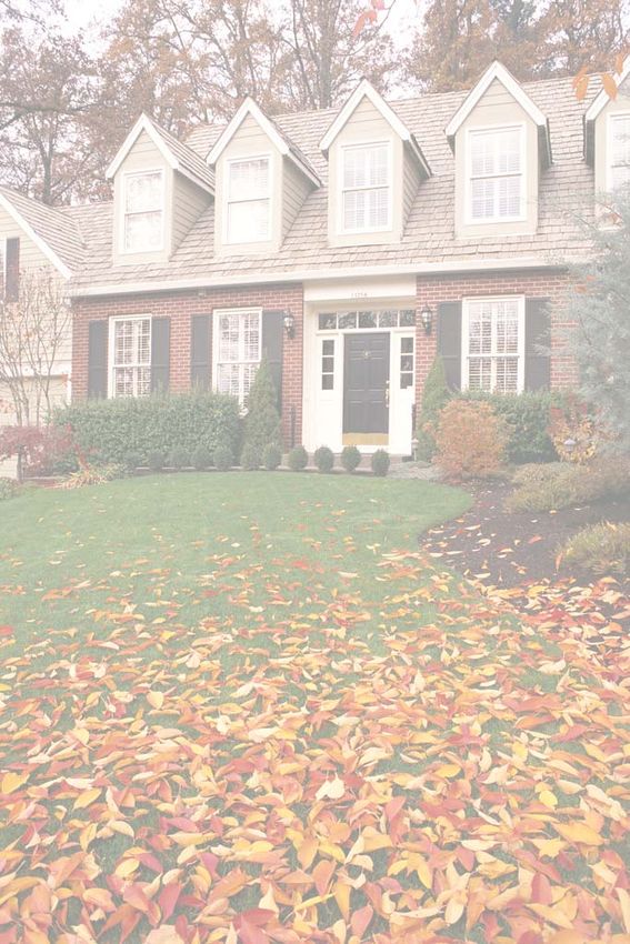
Census Bureau and the Tax Foundation; state household densities, by MSA, from the U.S. Census Bureau.Figure 6: Projected Economic Costs of the Subprime Mortgage Crisis State-by-State
W A: $
1,766
,842,1
92
MN: $1,640,695,039 395
99 ,8 1 0 ,
M E : $2
12
ID: $28
8, 7 91,0
OR: $ 6,895,7
09 WI: $855,191,927 $46
8 5 9 ,4
3 0 ,9 8 NH :
4 , 817 1
: $ 9 ,5 17,908 3
50,570 N Y 35, 139,0
MI: $3,121,4 $ 3 ,0
33 MA :
55,171,3
JOINT ECONOMIC COMMITTEE
N V : $1 IA: $260,762,474 PA: $2,4 ,0 5 3
,688,1
76,474 $ 6 69 ,5 9 4
R I:
25,370,9 27 326
UT: $614 IL: $5,400,921,912 OH: $3,7 , 4 2 4 ,600 ,
CA : $ ,9 91,567 1
23,78 C T: $
4,383 ,152 5, 019
,6 13 IN: $1,384,315 $ 6 , 4 0 5 ,9 2
NJ:
MO: $806,155,756 7,382 71
KY: $508,01 38 51 ,716,9
CO: $1,791,337
,694 ,2 12,421,2 2 , 7
V A : $ 2 MD: $
55
: $ 1,146,801,7 ,5 1 0
N C $ 2 5 7 ,1 5 2
AZ: $2,8 ,292 D C:
67,041,1
2 TN: $711,932
8 ,899,244
OK: $321,543,693 SC: $781
MS: $234,961,581
41
22,254,9
GA: $2,0
TX: $2,690,956,085 70
AL: $309,742,3
Total Economic Costs (Q3 2007-Q4 2009):
• Loss in Home Value
• Loss in Neighboring Property Values LA: $497,943,437
18 ,396,856
• Loss in Property Tax Revenues FL: $12,2
$13 Million to $230 Million $740 Million to $2.2 Billion
$230 Million to $740 Million $2.2 Billion to $24 Billion
OCTOBER 2007
Source: JEC Calculations.OCTOBER 2007 JOINT ECONOMIC COMMITTEE
Figure 7: State-Level Foreclosure Rate Regressions
Dependent Variable
Independent
Variable Foreclosure Rate
Foreclosure Rate ARM
FRM
House Price
-14.80 ** -9.27 **
Appreciation
(2004-2006) (2.058) (1.655)
Employment Growth -19.22 ** -11.19 *
(2004-2006) (5.930) (5.384)
Constant 8.88 ** 5.42 **
(0.570) (0.523)
Observations 51 51
2
R 0.712 0.490
* Significant at 95% level.
** Significant at 99% level.
Data Sources: Foreclosure rate are Mortgage Bankers Association “foreclosure inventory”; House Price Appreciation is calcu-
lated from Office of Federal Housing Enterprise Oversight housing price indices; Employment Growth is calculated from Bureau
of Labor Statistics “employees on non-farm payrolls,” seasonally adjusted. All data accessed via Haver Analytics.
closed within a year. Although there are variations across jurisdictions, the average maximum
amount of time to foreclose is less than a year.31
To estimate the numbers of mortgages that will be foreclosed, we begin by examining what
determines the fraction of mortgages in foreclosure (foreclosure rate) during a year. It is rea-
sonable to suppose that, holding the risk characteristics of borrowers constant, the foreclosure
rate will depend heavily on house price appreciation and the economic fortunes of borrow-
ers.32 If house prices appreciate, refinance or sale is easier. If general economic conditions
are good, it is more likely that households will be able to meet their financial commitments.
As it turns out, both these factors are significant determinants of the foreclosure rate. Figure 7
shows the results of state-level cross sectional regressions of subprime foreclosure rates for
2006 on two independent variables – cumulative housing price appreciation between 2004
and 2006, and cumulative employment growth in the same period. The cumulative housing
price appreciation variable is an index of changes in home equity, and the cumulative employ-
ment growth variable is an index of the ease of finding employment and the overall perform-
ance of the real economy. Both variables are statistically significant. The significance of the
employment variable highlights the importance of developments in the real economy for loan
outcomes. However, we do not attempt to estimate changes in employment when we use
these results. If employment growth were to slow during our forecast period, foreclosure
rates likely would be higher than our estimates.
To estimate future foreclosure rates, we use current foreclosure rates, the coefficients on
house price appreciation reported in Figure 7, and estimates of future housing prices. That is,
we calculate foreclosure rates according to FCt = FCt-1 + β(ΔHPAt), where FCt is the foreclo-
sure rate in year t, FCt-1 is the foreclosure rate in the previous year, ΔHPAt is the change in
15JOINT ECONOMIC COMMITTEE OCTOBER 2007
cumulative two-year housing price appreciation between years t and t-1, and β is the esti-
mated coefficient of HPA (house price appreciation) as reported in Figure 7. The values for
the variable ΔHPAt are calculated using forecasts of state-level housing price indices from the
Office of Federal Housing Enterprise Oversight (OFHEO). The forecasts were produced by
Moody’s Economy.com. We estimate foreclosure rates separately for fixed rate and adjust-
able rate mortgages. These foreclosure rates are used to calculate the absolute number of
foreclosures in a given period. 33
Using our estimates of the number of subprime foreclosures, we then estimate the associated
economic costs. Research has shown that foreclosure causes a decrease in the value of the
foreclosed house.34 We estimate this direct loss in housing wealth by discounting the average
loan value of a subprime mortgage. We apply a 22 percent discount rate to the average home
value associated with subprime loans (net of the loss due to the decline in home prices) to cal-
culate this loss. 35
Foreclosures also affect the values of neighboring houses. We estimate the effect of a fore-
closure on surrounding house prices as 0.9 percent of the value of all single family houses
within 1/8th mile of a foreclosed house.36 We use MSA-level population densities to estimate
the number of houses within one-eighth mile of each foreclosed house.37
The loss in property taxes caused by housing price losses is calculated by assuming that aver-
age state property tax rates remain unchanged through the end of 2009. Tax losses are calcu-
lated by applying existing property tax rates to the change in housing values caused by fore-
closure (net of the loss due to the decline in home prices).
We conclude by noting that the forecast values for housing prices clearly play a pivotal role in
this analysis, and that the price forecasts we have used are likely to be conservative. The
Moody’s data are forecasts of future values of OFHEO housing price indices. However, in
recent quarters the OFHEO indices have not reflected the same downward movement in hous-
ing prices registered in other price measures. For example, the national OFHEO index had
not peaked by the second quarter of 2007, but the S&P/Case-Shiller® U.S. national home
price index peaked in the second quarter of 2006 and had declined by 3.2 percent by the end
of the second quarter of 2007. Therefore it is possible that the price forecasts we have used
will not pick up all of the likely housing price declines over the near term.
To account for this possibility, we have applied the procedure developed for state level esti-
mates to aggregate foreclosures, assuming a 20 percent decline in aggregate home prices. A
price decline of that amount is not out of the question. When simulating the possible macro-
economic effects of housing price declines, the Federal Reserve recently assumed a 20 per-
cent decline in aggregate housing prices.38 Moreover, futures contracts based on the S&P/
Case-Shiller® indices are predicting that housing prices may decline as much as 10 percent
over the coming year.39 Since the S&P/Case-Shiller® indices already show a 3.2 percent de-
cline over the past year, calculating subprime foreclosures by assuming a 20 percent decline
in the OFHEO price indices over two years seems unfortunately plausible. Under these as-
sumptions, the number of foreclosures for the period covering the third quarter of 2007
through the end of 2009 is approximately 1.66 million, and the associated property loss
is about $106 billion.40 If we add in an estimate of foreclosures in the first half of 2007,
the foreclosure total rises to approximately 2 million.
16OCTOBER 2007 JOINT ECONOMIC COMMITTEE
Part III: The Origins of the Subprime Lending
Crisis
The discussion above highlights the potential economic damage that could result if subprime
foreclosures are allowed to proceed unchecked. In this section we investigate the underlying
causes of the subprime mortgage crisis in an effort to identify policy approaches that could
prevent the reoccurrence of such a threat to homeownership, household wealth, and the
broader economy.
FINANCIAL INTERMEDIARIES DROVE THE EXPANSION OF THE SUB-
PRIME MARKET
Most Lending Organizations Make Few Subprime Loans
The expansion of subprime mortgages during the years 2001 through 2006 came, for the most
part, through a well defined channel of financial intermediaries. The intermediaries in this
channel – brokers, mortgage companies, and the firms that securitize these mortgages and sell
them on to the capital markets – had strong incentives to increase the supply of these loans.
One outcome was a significant increase in the rate of homeownership. From 1994 to 2005,
the overall homeownership rate rose from 64 to 69 percent.41 However, since brokers and
mortgage companies are only weakly regulated, another outcome was a marked increase
in abusive and predatory lending.
Most Subprime Loans Are Originated Through Mortgage Brokers
The mortgages underwritten by subprime lenders come from many sources, but the over-
whelming majority is originated through mortgage brokers. For 2006, Inside Mortgage Fi-
nance estimates that 63.3 percent of all subprime originations came through brokers, with
19.4 percent coming through retail channels, and the remaining 17.4 percent through corre-
spondent lenders.42 Their data show the broker share increasing from 2003 through 2006.43,44
For the mortgage market in total, Inside Mortgage Finance estimates that 29.4 percent of
mortgages were originated by brokers in 2006. This percentage does not change much be-
tween 2003 and 2006.45
Independent Mortgage Companies and Other Mortgage Specialists Ac-
count for Most Subprime Lending
Most subprime loans are made by companies that specialize in mortgage lending. Using 2005
Home Mortgage Disclosure Act (HMDA) data, former Federal Reserve Governor Edward
Gramlich concluded that “30 percent of [subprime] loans are made by subsidiaries of banks
and thrifts, less [sic] lightly supervised than their parent company, and 50 percent are made by
independent mortgage companies, state-chartered but not subject to much federal supervision
at all.”46
17JOINT ECONOMIC COMMITTEE OCTOBER 2007
Figure 8: Mortgage Origination Statistics
Subprime Share in Percent Subprimes
Total Mortgage Subprime Subprime Mortgage
Total Originations Securitized
Originations Originations Backed Securities
(percent of dollar (percent of dollar
(Billions) (Billions) (Billions)
value) value)
2001 $2,215 $190 8.6 $95 50.4
2002 $2,885 $231 8.0 $121 52.7
2003 $3,945 $335 8.5 $202 60.5
2004 $2,920 $540 18.5 $401 74.3
2005 $3,120 $625 20.0 $507 81.2
2006 $2,980 $600 20.1 $483 80.5
Source: Inside Mortgage Finance, The 2007 Mortgage Market Statistical Annual, Top Subprime Mortgage Market Players &
Key Data (2006).
Because they are not deposit-taking institutions, the independent mortgage companies
and bank subsidiaries are not subject to the safety and soundness regulations that gov-
ern federal or state banks. These entities are less closely monitored under the Home Own-
ers’ Equity Protection Act (HOEPA) and the Community Reinvestment Act. They are state-
chartered and subject to state law. Some states have tried to apply federal predatory lending
advisories to all lenders or regulate brokers or lenders in their state, but the resources that
states have for oversight are far fewer than those of the federal government.47
Most Subprime Loans are Securitized Via Non-Agency Conduits to the
Capital Markets
Lenders hold only a fraction of the subprime loans they make in their own portfolios. Most
are sold to the secondary market, where they are pooled and become the underlying assets for
residential mortgage backed securities. As can be seen from the data in Figure 8, the percent-
age of subprime mortgage securitized rose rapidly after 2001, reaching a peak value of more
than 81 percent in 2005. Deposit-taking institutions such as banks and thrifts, which deal
mostly in lower-priced mortgages, sell their mortgages primarily to government sponsored
enterprises (GSEs) such as Fannie Mae and Freddie Mac. Independent mortgage companies,
however, make their secondary market sales primarily to other financial market outlets (See
Figure 9).48 Hence whatever influence the GSEs have on lender underwriting standards
is missing from much of the subprime market since securitization is done by other mar-
ket participants.
18OCTOBER 2007 JOINT ECONOMIC COMMITTEE
Figure 9: Subprime Lenders Usually Securitize Loans Through Non-GSE Conduits
Percent Distribution
Higher-Priced Specialized Lender
Percent Sold in 2004
Bank or Mortgage Affiliate Other
Not Sold GSE Private Total
Thrift Company Institution Conduits
Deposit Taking Organizations
Credit Unions 0.4 0.0 0.0 0.0 0.0 0.0 0.0 0.5
CRA-Regulated Lenders
Assessment Area Lenders 1.4 0.0 0.0 0.1 0.0 0.0 1.0 2.6
Outside Assessment Area 4.1 0.0 0.0 0.7 0.0 0.3 8.3 13.5
Independent Mortgage Bankers 12.6 0.1 1.7 0.6 12.4 1.6 54.4 83.4
All Loans 18.4 0.1 1.7 1.5 12.5 1.9 63.8 100.0
Lower-Priced Specialized Lender
Percent Sold in 2004
Bank or Mortgage Affiliate Other
Not Sold GSE Private Total
Thrift Company Institution Conduits
Deposit Taking Organizations
Credit Unions 5.6 1.3 0.0 0.1 0.3 0.1 0.4 7.8
CRA-Regulated Lenders
Assessment Area Lenders 18.8 11.6 0.0 0.9 0.5 2.3 2.9 37.0
Outside Assessment Area 8.6 10.1 0.1 1.0 1.0 2.8 5.4 29.0
Independent Mortgage Bankers 1.5 5.6 0.5 2.1 6.0 0.2 10.4 26.2
All Loans 34.5 28.5 0.6 4.0 7.8 5.5 19.1 100.0
Source: Apgar, et al. 2007.
Note: Higher-Priced Specialized Lenders are, approximately, firms that specialized in subprime lending. Lower-Priced Specialized
Lenders tend to make few subprime loans. See the discussion in Apgar et al. (2007).
19JOINT ECONOMIC COMMITTEE OCTOBER 2007
MARKET INCENTIVES FACILITATED PREDATORY LENDING
Broker and Lender Incentives Work Against Borrowers
Mortgage brokers are salesmen who want to maximize their net income. Their interest in pro-
viding the least expensive mortgage is limited. In fact, lenders provide them incentives to do
the opposite. Lenders sometimes pay brokers so-called “yield-spread premiums,” when they
sell loans with interest rates above the minimum acceptable rate for the loan.49 Some brokers
may also receive higher fees for selling mortgages with prepayment penalties.50
Moreover, since mortgage brokers bear little or no risk when a borrower defaults, they
have no economic incentive to originate loans that a borrower can afford in the long
term. Brokers also lack strong legal incentives to act in the interest of borrowers. Under
state law brokers are not fiduciaries, who must put the interest of their clients first. Nor do
they have a duty to sell their clients products which are at least suitable to their circumstances,
as registered securities brokers do.
Because mortgage companies sell many of the loans they underwrite to the secondary
market, they have an interest in underwriting loans that are desired by the secondary
market investors.51 This observation has special weight because of developments in non-
mortgage financial markets. In recent years, as hedge funds have proliferated and the market
for structured financial products has expanded, there has been significant demand for high-
yield assets that can underlie collateralized debt obligations (CDOs) and other financial de-
rivatives. Subprime mortgages have, until recently, been considered terrific assets to include
in CDO structures. Hence subprime lenders have had a strong incentive to underwrite
high-yielding subprime mortgages, whether or not these loans were best interests of the
borrowers.
Predatory Lending Practices
Given the financial incentives for brokers and lenders to provide an increasing volume of high
yield mortgages, it is no surprise that tactics were invented to meet the demand. The rapid
expansion of 2/28 and 3/27 hybrid ARMs, and the imposition of prepayment penalties, are
examples of financial innovations that were widely adopted by subprime lenders.52 Both
made it possible for loan originators to expand lending—hybrid ARMs by allowing credit-
constrained borrowers to pay initially low rates on mortgages, and prepayment penalties by
raising returns on loans. However, both innovations can have abusive or predatory results.
In the abstract, ARM loans need not work to the disadvantage of borrowers. Subprime hybrid
ARMs, however, have frequently been made on the basis of the borrower’s ability to pay at
the low initial rate rather than the reset rate. This is reflected in public disclosures of lenders,
who make it clear that they qualify borrowers for loans on the basis of their ability to make
payments at or near the initial rate.53 It is also reflected in loan performance. When hybrids
reset there is a dramatic rise in prepayments as borrowers refinance and an increase in the de-
fault rate. Prepayments and defaults are very sensitive to the size of these shocks. Penning-
ton-Cross and Ho estimate that “a one-standard-deviation increase in the size of the shock is
associated with an almost 50 percent increase in the probability of prepaying and more than a
20OCTOBER 2007 JOINT ECONOMIC COMMITTEE
Figure 10: Underwriting Standards in Subprime Home-Purchase Loans
Low-No-Doc Debt Payments- Average Loan-
ARM Share IO Share
Share to-Income Ratio to-Value Ratio
2001 73.8% 0.0% 28.5% 39.7 84.04
2002 80.0% 2.3% 38.6% 40.1 84.42
2003 80.1% 8.6% 42.8% 40.5 86.09
2004 89.4% 27.2% 45.2% 41.2 84.86
2005 93.3% 37.8% 50.7% 41.8 83.24
2006 91.3% 22.8% 50.8% 42.4 83.35
Source: Freddie Mac, obtained from the International Monetary Fund via http://www.imf.org/external/pubs/ft/fmu/eng/2007/
charts.pdf.
Notes: “ARM” represents “adjustable rate mortgages”; “IO” represents interest-only mortgages, where payments do not retire the
principal value of the loan; “Low-No-Doc” represents low or no documentation mortgages.
25 percent increase in the probability of defaulting.”54 By underwriting hybrid loans on the
basis of the initial rate, lenders make it more probable that a subprime borrower must
sell, refinance or default at reset. This means there is increased lender reliance on asset val-
ues and prepayment fees to provide earnings, and less consideration of borrower ability to
pay.
Mortgage lending on the basis of asset value, without regard to borrower ability to pay,
is widely recognized as predatory and harmful to borrowers. HOEPA recognizes asset-
based mortgage lending as predatory, as do several state statutes.55 Several researchers also
regard asset-based mortgages as predatory.56 However, HOEPA coverage is limited. Because
HOEPA applies only to loans that have an annual percentage rate that exceeds a very high
threshold, less than one percent of subprime loans are covered.57 Currently at least 41 states
have laws which restrict predatory mortgage lending, but the terms and enforcement of these
statutes are uneven.58
Moreover, unscrupulous originators can evade state law by falsifying information or making
“no documentation” loans that make loans appear affordable even when they are not.59 The
remarkable expansion of low document and no document loans, observable in Figure 10, is
likely to reflect something more than risk-taking by lenders. It may also measure the determi-
nation of originators to evade state controls on predatory lending.
Prepayment penalties, which are frequently imposed on all types of subprime loans at a very
high relative and absolute rate (See Figure 15), have the potential to strip housing equity from
subprime borrowers. As Farris and Richardson note: “The typical penalty is six months’ in-
21You can also read