Classical Nuclear Motion: Comparison to Approaches with Quantum Mechanical Nuclear Motion - MDPI
←
→
Page content transcription
If your browser does not render page correctly, please read the page content below
Article
Classical Nuclear Motion: Comparison to Approaches with
Quantum Mechanical Nuclear Motion
Irmgard Frank

                                         Institute of Physical Chemistry and Electrochemistry, Theoretical Chemistry, Leibniz University of Hannover,
                                         Callinstr. 3A, 30167 Hannover, Germany; irmgard.frank@theochem.uni-hannover.de

                                         Abstract: Ab initio molecular dynamics combines a classical description of nuclear motion with
                                         a density-functional description of the electronic cloud. This approach nicely describes chemical
                                         reactions. A possible conclusion is that a quantum mechanical description of nuclear motion is not
                                         needed. Using Occam’s razor, this means that, being the simpler approach, classical nuclear motion
                                         is preferable. In this paper, it is claimed that nuclear motion is classical, and this hypothesis will be
                                         tested in comparison to methods with quantum mechanical nuclear motion. In particular, we apply
                                         ab initio molecular dynamics to two photoreactions involving hydrogen. Hydrogen, as the lightest
                                         element, is often assumed to show quantum mechanical tunneling. We will see that the classical
                                         picture is fully sufficient. The quantum mechanical view leads to phenomena that are difficult to
                                         understand, such as the entanglement of nuclear motion. In contrast, it is easy to understand the
                                         simple classical picture which assumes that nuclear motion is steady and uniform unless a force is
                                         acting. Of course, such a hypothesis must be verified for many systems and phenomena, and this
                                         paper is one more step in this direction.

                                         Keywords: Car–Parrinello molecular dynamics; chemical reactions; photoreactions; classical
                                         nuclear motion

                                         1. Introduction
                                              What led us to describing nuclear motion classically in simulations of chemical reac-
Citation: Frank, I. Classical Nuclear    tions [1–3]. It all started with the famous publication of Car and Parrinello [4]: “Unified
Motion: Comparison to Approaches         Approach for Molecular Dynamics and Density-Functional Theory”. In their seminal work,
with Quantum Mechanical Nuclear
                                         Car and Parrinello started from the Born–Oppenheimer approximation to “separate nuclear
Motion. Hydrogen 2023, 4, 11–21.
                                         and electronic coordinates” [4]. With this understatement, the resulting method is what
https://doi.org/10.3390/
                                         sometimes is called semiclassical: density functional theory (DFT) for the electrons and
hydrogen4010002
                                         a classical treatment for the nuclei (it should be mentioned that the general idea was in
Academic Editor: Jacques Huot            the world before; see the Nobel prize lecture of Karplus). While being deterministic, the
                                         approach of Car and Parrinello is different from Bohm mechanics, which merely reformu-
Received: 23 October 2022
                                         lates Schrödinger’s theory. Instead of a “guiding equation”, as in Bohm’s theory, we have
Revised: 26 November 2022
Accepted: 19 December 2022
                                         simply Newton’s equation.
Published: 29 December 2022
                                              Car and Parrinello constructed an extended Lagrangian and made it possible to use this
                                         idea in a working code. They developed a numerically extremely successful concept: density
                                         functionals at the generalized gradient approximation (GGA) level/pseudopotentials for the
                                         inner electrons/periodic boundary conditions/plane waves for the valence electrons/Car–
Copyright:   © 2022 by the author.       Parrinello equations for electronic motion. This approach is efficient for several reasons:
Licensee MDPI, Basel, Switzerland.       1. The use of plane waves makes it possible to perform simulations with changing atomic
This article is an open access article   distances without a basis superposition error and without Pulay forces, that is, we obtain
distributed under the terms and          no additional terms by pulling basis functions through space. 2. If huge plane-wave basis
conditions of the Creative Commons
                                         sets are used, we are essentially restricted to GGA functionals. Hybrid functionals are too
Attribution (CC BY) license (https://
                                         expensive due to the use of Hartree–Fock exchange. 3. Pseudopotentials make the plane-
creativecommons.org/licenses/by/
                                         wave basis sets tractable. This results in almost complete basis sets for the valence electrons.
4.0/).

Hydrogen 2023, 4, 11–21. https://doi.org/10.3390/hydrogen4010002                                           https://www.mdpi.com/journal/hydrogen
Hydrogen 2023, 4                                                                                               12

                         At the start of a Car–Parrinello molecular dynamics (CPMD) simulation, the electronic
                   structure is computed using density functional theory. During the simulation, it is prop-
                   agated using the Car–Parrinello equations. These equations include an additional term
                   which contains the forces on the electronic cloud, that is, the second derivatives of the
                   orbitals multiplied by a fictitious electron mass. It is unpleasant to need such a parameter as
                   the fictitious electron mass, but this parameter can be varied over two orders of magnitude
                   without a strong change. By setting it to about 400–500 atomic units instead of 1 atomic
                   unit, it is possible to save CPU time. The result works excellently. This may be explained
                   by the beauty of the Car–Parrinello equations: we have second derivatives for both space
                   and time. It is a purely deterministic approach that can be solved numerically, time step by
                   time step, using Equation (5a,b) in Ref. [4]. Time steps are introduced during which the
                   forces can be assumed as constant. They have typical values of about 0.1 fs. Normally, this
                   leads to stable dynamics. The implementation of the Car–Parrinello equations is not easy;
                   hence, not so many implementations exist. The most famous is the CPMD code written
                   by Hutter et al. [5], which is extremely well parallelized and is also very user-friendly.
                   The CPMD code also contains an implementation of what is called Born–Oppenheimer
                   dynamics (BOMD), namely, molecular dynamics with full optimization of the electronic
                   wave function in every time step instead of a CP molecular dynamics. Both BOMD and
                   CPMD are summarized as ab initio molecular dynamics (AIMD). BOMD is almost one
                   order of magnitude slower than CPMD, depending on the time step chosen. Since in BOMD
                   simulations the motion of the electrons does not have to be resolved, a larger time step
                   (0.1–0.5 fs) than in CPMD simulations (0.05–0.1 fs) may be used. Using a too-large time
                   step leads to a drift of the total energy (see Supplementary Material, Figures S1–S5).
                         The approach to compute only the points that are reached during dynamics, instead
                   of calculating a complete potential energy surface, is called “on the fly” simulations. Two
                   simulations starting from the same initial conditions will always lead to the same re-
                   sult. Slightly changing the initial conditions can lead to different products, that is, we
                   have deterministic chaos but no quantum chaos. Since the velocities of the atoms are
                   Maxwell–Boltzmann-distributed, there is no classically forbidden region [3]. We do not
                   have to do anything to achieve this distribution. It develops automatically in a molecular
                   dynamics run as it is the most likely distribution. The fastest parts of a molecular system
                   may undergo chemical reactions.
                         One more point that should be mentioned is the kinetic isotope effect: in contrast to
                   the static isotope effect, it can normally be measured. When using Newton dynamics, this is
                   explained by the fact that the force depends on the mass, F = m a. In contrast, static isotope
                   effects that depend on the zero-point energy cannot be observed. While there is a lot of
                   zero-point energy in the electronic wave function of every atom due to the 1/r potential,
                   there is no zero-point energy in nuclear motion. This facilitates the understanding of matter
                   at low energies: near-zero-Kelvin nuclei hardly move, while the electrons form a static
                   cloud that cannot be compressed much stronger.
                         In the present paper, I will compare CPMD and BOMD results, as obtained with the
                   CPMD code, to the pioneering work of Marx [6–9], Domcke [10–13], Hammes-Schiffer [14],
                   Martinez [15,16], and coworkers, certainly ignoring many others (for a review, see, for
                   example, Ref. [11]). It is the experience from these excellent studies that leads to the
                   thought that a quantum mechanical description of nuclear motion is not needed. For the
                   excited states I will use restricted open-shell Kohn–Sham (ROKS) calculations [17]. Hereby,
                   ROKS is merely an approach that solves the electronic structure problem for excited states
                   self-consistently with minimum computational effort at the DFT level of accuracy. An
                   interesting feature of ROKS is that, as a single-configuration method, it is diabatic. We
                   use the single electronic configuration that describes a pure HOMO–LUMO transition.
                   During a chemical reaction, for example, a dissociation, this configuration may become the
                   open-shell ground state. Alternatives are real-time TDDFT methods [18–22], which use
                   time-dependent DFT in their original meaning, without using perturbation theory. This
                   field is still in development. Of course, time-dependent DFT also describes the electronic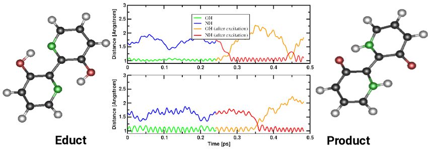
Hydrogen 2023, 4                                                                                               13

                   wave function only. Similar to other quantum chemical excited-state methods, it can be
                   combined with classical or quantum mechanical nuclear motion.

                   2. Methods
                         Using the CPMD code, ab initio molecular dynamics simulations [4,5,23] were per-
                   formed in the NVE ensemble using the Becke–Lee–Yang–Parr (BLYP) functional in con-
                   nection with the Grimme dispersion correction [24]. The wave function was optimized
                   in every time step (“Born–Oppenheimer molecular dynamics”). For comparison, some
                   calculations were performed with Car–Parrinello molecular dynamics. The time step was
                   chosen as 5 a.u. (0.1209 fs). This time step is relatively small for BOMD simulations and
                   was chosen in order to describe the excited state as accurately as possible. Troullier–Martins
                   pseudopotentials, as optimized for the BLYP functional, were employed for describing the
                   core electrons [25,26]. The plane-wave cutoff, which determines the size of the basis set, was
                   set to 70.0 Rydberg. This corresponds to a very large basis set. In the case of the phenol pho-
                   todissociation, the simulation cell size was 14 × 14 × 14 a.u.3 (7.4 × 7.4 × 7.4 Angstrom).
                   For the orbital plots, a cell size of 18 × 18 × 18 a.u.3 (9.5 × 9.5 × 9.5 Angstrom) was chosen
                   in order to account for the diffuse character of the LUMO in the Franck–Condon region.
                   After geometry optimization, an equilibration in the ground state was performed, with
                   initial temperatures ranging from 0 to 2000 K. During the equilibration, half of this initial
                   kinetic energy is converted into potential energy, leading to temperatures that are only
                   half as high. The kinetic energy distribution was chosen in this way in order to model a
                   Maxwell–Boltzmann distribution, which permits high energies of single particles. In the
                   ground state, the molecules are stable under these conditions on the picosecond timescale.
                   After equilibration, the system was placed vertically into the excited state by changing
                   the occupation pattern (restricted open-shell Kohn–Sham, ROKS [17]) while keeping the
                   ground-state velocities.
                         The same protocol was used for bipyridyl systems, except that the simulation cell was
                   always kept at 18 × 18 × 18 a.u.3 (9.5 × 9.5 × 9.5 Angstrom). The initial kinetic energies
                   were varied between 600 and 2400 K.
                         For comparison, CPMD simulations were performed (see the Supplementary Material).
                   The time step was chosen as 2 a.u. (0.048 fs), and the fictitious electron mass as 200 a.u.

                   3. Results
                   3.1. Wave Packets and Alternatives
                        The Schrödinger equation for any system composed of atoms reads:

                                                           Ĥtotal Ψ = Etotal Ψ                               (1)

                                         Ĥtotal = T̂nuc + T̂el + V̂nuc−nuc + V̂nuc−el + V̂el −el             (2)
                        The Hamilton operator contains all kinetic and potential energy terms: the kinetic
                   energies of nuclei and electrons plus the nuclear–nuclear interactions, the nuclear–electronic
                   interactions, and the electronic–electronic interactions. At this point, normally, the Born–
                   Oppenheimer approximation is applied, separating the electronic problem in the electronic
                   Hamilton operator:
                                                    Ĥel = T̂el + V̂nuc−el + V̂el −el                         (3)
                        Applying density functional theory (or other approximations to the electronic prob-
                   lem) to ground and excited states of a molecular system yields what is known as Born–
                   Oppenheimer surfaces or also potential energy surfaces. For covalent interactions, Morse
                   potentials are obtained. This, however, works only if the nuclear–nuclear interaction is
                   added to the energy computed for the electronic Hamiltonian. This is no small correc-
                   tion: if the nuclear–nuclear interaction is omitted, the nuclei collapse to a distance of zero
                   Angstrom. Without the nuclear repulsion, the minimum of the Morse potential, which
                   keeps the nuclei at a distance, disappears. Hence, the total energy in a normal quantum
Hydrogen 2023, 4                                                                                                        14

                   chemical calculation contains the kinetic energy of the electrons, the electron–electron
                   interaction, the electron–nuclear interaction, and the nuclear–nuclear interaction:

                                               ĤQC = T̂el + V̂nuc−nuc + V̂nuc−el + V̂el −el                            (4)

                        The only term missing is the kinetic energy of the nuclei. This corresponds to the
                   situation at zero Kelvin. Hence, normal quantum chemical calculations are performed at
                   zero Kelvin. This changes if ab initio molecular dynamics is employed: then, the kinetic
                   energy of the nuclei is replaced by the classical term. The structure or motion of the nuclei
                   does not play any role in quantum chemical calculations. By good luck, the structural
                   differences between zero Kelvin and room temperature are normally small in molecular
                   systems. Hence, we know how to compute potential energy surfaces: not by introducing
                   a product ansatz and a separation of variables, but by setting the temperature of the
                   nuclear system to zero. It is consistent to treat the nuclei as classical particles right from the
                   beginning as practiced in AIMD simulations. As a result, we have a wave function for the
                   electrons only, no product ansatz, and no separation of variables. All five energy terms act
                   on this electronic wave function:

                         Ĥ AI MD Ψel = ( T̂nuc,classical + T̂el + V̂nuc−nuc + V̂nuc−el + V̂el −el )Ψel = E AI MD Ψel   (5)

                        In the SCF calculation, only the three of them which are contained in Ĥel matter. The
                   two remaining energy terms are added after the SCF or, in a CPMD simulation, once in
                   every time step. The nuclear–nuclear interaction is simply the electrostatic interaction of
                   classical point particles.
                        Taking derivatives of the total energy expression Ĥ AI MD with respect to the classical
                   nuclei, we obtain the following classical equation for the nuclei:

                                                                           ∂
                                                           M I R̈ I = −       E                                         (6)
                                                                          ∂R I QC

                         Capital letters are used for the nuclei. In addition, this equation for the nuclei contains
                   all five terms: on the left side, we have the derivative of the classical kinetic energy, that is,
                   the accelerations or forces; on the right side, we have the derivative of EQC which contains
                   the remaining four terms.
                         As is known from experiments, nuclei have a certain size, which is in the region of a
                   few femtometers. There is no theoretical approach which would yield this size in a reliable
                   way, such as the electronic Schrödinger equation reliably yielding the extension of the
                   electronic cloud. We can explain the periodic system, but not the isotope chart. Within
                   the isotope chart, the density of the nuclei is almost constant; hence, they do not become
                   smaller with increasing mass. A naive application of the deBroglie theory of matter waves
                   would yield a wrong result. Similar to any massive object, the mass, and not the size, of a
                   particle determines the motion of its center of mass.
                         Let us return to the potential energy surfaces. It is a wide and well-established field
                   of research to compute these surfaces with standard quantum chemical methods and, in
                   a second step, to model the nuclear situation using wave packet approaches. However,
                   these wave packets are too large, by several orders of magnitude, to be related to the
                   structure of a nucleus. Nuclear wave packets may spread and recombine, which, however,
                   is not interpreted as nuclear fission or fusion. It is, rather, assumed that the nuclear wave
                   function is smeared out and that this can be healed by a measurement, eventually leading
                   to different chemical products; however, such a smeared nuclear wave function (or, rather,
                   its density) is never observed in experiment. There is no reason to give up the Rutherford
                   picture of tiny nuclei, which are larger the heavier the nucleus is. Nowadays, with large
                   computers, it may seem the better alternative to switch to classical many-body theory for
                   nuclear motion instead of investigating wave packets in a few dimensions.
                         What about photoreactions? In addition, in this context, what about branching at
                   conical intersections? It is certainly true that conical intersections are everywhere [27];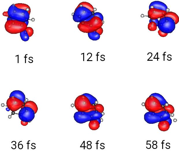
Hydrogen 2023, 4 15
however, they are far less responsible for the outcome of a photoreaction than the dynamics
in the Franck–Condon region which may lead the way to different conical intersections [28].
An example is the photochemistry of CH3 Cl [2]. Immediately after excitation, the system
may decide in which direction to move: either C–Cl dissociation or C–H dissociation.
The conical intersections for both reaction paths are reached much later. If, similar to the
restricted open-shell Kohn–Sham (ROKS) method [17], a diabatic method is used, the nuclei
do not behave strangely at these conical intersections. In the single-configuration ROKS
picture, which is diabatic by construction, the nuclei simply accelerate while the system is
reaching lower regions of the potential energy surface. They do not branch, nor do they
show any other strange behavior at the diabatic crossings. It was also shown for pyrrole
that this is sufficient to explain the experiment [29]: there is a shallow minimum near
the Franck–Condon region which causes a second reaction channel. This second reaction
channel is not due to the motion near the conical intersection, which is reached later.
ROKS yields excited-state gradients in a straightforward way using the Hellmann–
Feynman theorem. Nevertheless, one might hope for a more versatile approach if extending
this to an adiabatic many-configuration ansatz followed by a nonadiabatic treatment. Sur-
face hopping does not solve the problem [13]. More interesting is the use of a diabatization
which, however, is not uniquely defined [30]. When making a comparison between wave-
packet and on-the-fly methods, the drawbacks of the on-the-fly methods must also be
emphasized. Of course, the diabatic ROKS method also has its shortcomings. In particular,
there is presently no convincing implementation which would allow for the use of hybrid
functionals. As a result, we typically obtain a vertical excitation energy which is too low by
about 0.6 eV, which we compensate by starting with higher kinetic energies. In addition,
similar to the case for any excited-state self-consistent field calculation, convergence is much
worse than for the ground state, and sometimes jumps in the total energy are observed.
Finally it is not possible at the moment to combine Car–Parrinello molecular dynamics and
ROKS. We are restricted to Born–Oppenheimer molecular dynamics simulations. Yet, this
does not affect nuclear motion, and the classical picture of nuclear motion survives.
In the present study, we apply ROKS/BLYP to the photoreaction of phenol, which
was studied before by Domcke and coworkers [10,12,31]. While in these wave-packet
calculations the average O–H distance reaches 3 Angstrom within 30 fs, we observe only
partial dissociation. In most simulations (7 out of 10), we observe no photoreaction at
all within 1.2 ps of simulation time. In the remaining cases, we observe the dissociation
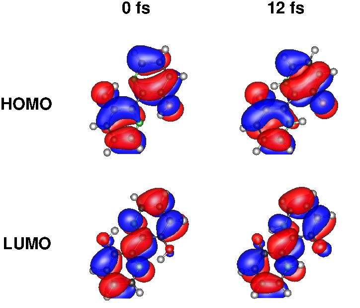
connected to the transformation of the LUMO to a 1s orbital, while the HOMO hardly
changes shape (Figures 1 and 2). The transformation is mostly smooth, but there is a
problem with the SCF about 0.02 ps after the excitation. The wave function suddenly
changes sign, which is accompanied by a slight jump in energy (see the Supplementary
Material, Figure S6). This is one of the disadvantages of Born–Oppenheimer molecular
dynamics compared to Car–Parrinello molecular dynamics: such sudden changes in an
SCF calculation are numerically possible. The same applies to the slight slope of the total
energy. In addition, here, Car–Parrinello molecular dynamics would be superior, even if
we use a very small time step (0.1 fs) in the Born–Oppenheimer dynamics simulations.
The reaction path observed consists mainly of the dissociation of the O–H bond. The
LUMO of phenol is transformed into the 1s orbital of the resulting hydrogen atom. As
can be seen in Figure 2, after 48 fs, the bond cleavage is supported by an interaction
with a neighboring hydrogen atom. With all the drawbacks of ROKS, we obtain a very
clear and convincing picture of the development of the electronic structure during this
photoreaction. The picture obtained by a wave-packet description [10] is also convincing.
While in the classical picture the observation of different outcomes is due to the dynamics in
the Franck–Condon region, the quantum mechanical picture attributes the branching to the
motion through conical intersections. One might mention, however, that in the quantum
mechanical description, the nuclear probability density of the product state is smeared over
several Angstrom, which is not necessarily a realistic picture.Hydrogen 2023, 4 16
Figure 1. HOMO of phenol during the photoreaction (ROKS simulation). Apart from a rapid change
of sign between 12 and 24 fs, not much happens to the electronic structure. A hydrogen atom is
expelled at the end of the simulation (at the right side of the molecule).
Figure 2. LUMO of phenol during the photoreaction (ROKS simulation). The motion starts from a π ∗
orbital which has already an antibinding interaction concerning the O–H bond. The elongation of
this bond leads to the formation of the 1s orbital of the dissociating hydrogen atom.
3.2. Multiple Spawning
Martinez and coworkers developed, very early, a quantum mechanical implementation
of nuclear motion. With multiple spawning, the situation in nonadiabatic regions, e.g.,
near a conical intersection, is described [15]. The authors already presented, in 1998,
an impressive application to the photoisomerization of retinal in bacteriorhodopsin [32].
A related problem, namely, the photoisomerization of retinal in bovine rhodopsin, was
studied with ROKS/BLYP using a QM/MM approach in order to model the protein
environment [33]. The ROKS study, using excited-state self-consistent field (SCF) theory,
produced the particularly nice result that of all double bonds in retinal which could
isomerize, only the C11 –C12 bond rotates upon excitation. This is due to the shape ofHydrogen 2023, 4 17
the binding pocket and to the location of the counterion. However, to be precise concerning
all advantages and disadvantages, it must be mentioned that a higher temperature had
to be applied to compensate for the ROKS/BLYP redshift. The result is one of still very
few unconstrained QM/MM simulations showing a chemical reaction in a protein on the
fly. In the multiple spawning calculations, the shape of the quantum mechanical nuclei
is strongly determined by Gaussian basis functions, and care must be taken not to obtain
complete delocalization. Again, the conceptionally simpler (but computationally way more
expensive) diabatic AIMD model with classical nuclear motion has some advantages. In
any case, also for protein chemistry, we find no reason to assume quantum effects in nuclear
motion. The experience from QM/MM calculations, rather, leads to the conclusion that
nuclear motion may be described in the same way for both the QM and the MM parts of
the system.
3.3. Path Integrals
A concept based on the work of Feynman is the use of path integrals. In the application
to molecular problems [6–9], multiple pathways are computed during a complete on-the-fly
simulation. Typically, ground state situations were treated. The implementation of path
integrals in the CPMD code made it possible to simulate fluxional molecules at this high
theoretical level; however, comparison to experiment does not prove at all that a quantum
description of nuclear motion is necessary. Temperature has a qualitatively similar effect.
More recently, it was shown that path-integral MD works far worse when applied to the
simulation of chemical reactions [2]. For example, in a dissociation reaction, the nuclear
clouds of both fragments stay entangled. It is not clear by what mechanism, and at what
point in time, that this entangled result could possibly be transformed again into reasonable
molecules. Feynman’s view of quantum mechanics was based on thought experiments [34].
It may be applied fruitfully in high-energy situations, but not in quantum chemistry.
Classical on-the-fly computations on large computers lead to a different picture.
3.4. Full Treatment
An important step towards a full treatment of both electronic and nuclear structure
was made by Hammes–Schiffer and coworkers [14,35,36]. In their nuclear-electronic orbital
(NEO) method, the authors do not make use of the Born–Oppenheimer separation, but
solve the complete problem straightforwardly. In numerical applications, however, only
the nuclei of the hydrogen atoms are selected for a quantum mechanical treatment. The
authors succeeded in programming analytic excited-state gradients, which facilitated the
computation of optimized geometries. For the description of the electronically excited
states, they used time-dependent density functional theory (TDDFT), respectively, the
combination NEO-TDDFT.
While this should be a powerful approach, it is observed that the nuclei are smeared
out over a distance that is much larger than 1 fm. It might be the choice of the Gaussian
basis set which keeps them at the size observed. The quantum mechanical treatment of
all the nuclei is computationally expensive. Yet, there might be yet another reason for not
computing all nuclei quantum-mechanically: if all nuclei are treated in this way, there
will be no external potential left, and both the electronic and the nuclear densities will be
smeared out. A critical test for the method, which does not cost too much CPU time, might
be the fully quantum mechanical simulation of hydrogen formation from two hydrogen
atoms, ideally using an unbiased plane-wave basis set [2].
In order to compare, we performed ROKS simulations for the 2,20 -bipyridine, [2,20 -
bipyridyl]-3-ol and [2,20 -bipyridyl]-3,30 -diol systems. The latter two substances were in-
vestigated by Hammes–Schiffer and coworkers. For bipyridyl-diol, we find an immediate
hydrogen transfer from the OH groups to the nitrogen atom. Movies of the two singly
occupied orbitals are added in the Supplementary Material. The mechanism corresponds to
an excited-state intramolecular proton transfer (ESIPT). The two proton transfers are almost
simultaneous (Figure 3). While this reaction is fast, we observe no rotation about the centralHydrogen 2023, 4 18
carbon–carbon bond [36]. This is no surprise: the lowest unoccupied molecular orbital
(LUMO), which is populated upon excitation, exhibits a binding interaction for the central
carbon–carbon bond (Figure 4). The same is true for bipyridine and bipyridyl-ol (Figure 5).
In the ROKS simulations, we observe no motion that would explain radiationless decay.
Near the excited-state minimum, we place the system back to the ground-state surface. This
is connected with a jump in energy (see the Supplementary Material, Figures S7 and S8).
This jump is due to the fact that we converge the wave function in every time step. A more
realistic picture of the electronic motion near the state crossing could be obtained if we
could use a CPMD-like approach, with a steady and continuous motion of all parts of the
system, instead of BOMD, with full convergence of the orbitals. This does not affect nuclear
motion; the ESIPT is described correctly.
Figure 3. Photoreaction of [2,20 -bipyridyl]-3,30 -diol, ROKS simulation. Upper and lower panel:
reaction of the two OH groups, respectively. The isomerization events, which are characterized by
a crossing of the orange and red curves, are not exactly simultaneous, but follow closely one after
the other. Color code of educt and product plots: white: hydrogen, black: carbon, green: nitrogen,
red: oxygen.
Figure 4. HOMO and LUMO of [2,20 -bipyridyl]-3,30 -diol before and after the photoreaction. The
central carbon–carbon bond is strengthened in the excited state and adopts double bond character.Hydrogen 2023, 4 19
Figure 5. (a) LUMO of [2,20 -bipyridyl]-3-ol; (b) LUMO of bipyridine. The LUMOs resemble the
LUMO of bipyridyl-diol. Upon occupation of this orbital, the central carbon–carbon bond is strength-
ened. This prevents a rotation.
4. Discussion
It is the state of the art to compute the electronic structure at the DFT level and nuclear
motion classically in an on-the-fly approach. The basis of this picture is a model that is
in agreement with the Rutherford atom model concerning the nuclei, while the electronic
structure is computed using the Schrödinger equation: tiny, positively charged nuclei are
surrounded by a negatively charged electronic cloud. In contrast to the electrons, the
nuclei (C, H, O, N, etc.) can be discriminated. This model ignores the possibility of nuclear
fusion and fission, i.e., the nuclei in our picture are perfectly stable. Obviously, we make
an approximation and we investigate if this approximation is superior to the quantum
mechanical picture of nuclear motion. In a classical description, there is no zero-point
energy in nuclear motion. This represents no problem since, due to the 1/r potential,
our bound electrons have infinite zero-point energy, which is more than enough. Very
obviously, the approach we use (Schrödinger equation for the electronic structure, Newton
dynamics for the nuclear motion) works for bound electrons only and is an approximation
to a more general field theory. It is not unlikely that such a more general field theory is
numerically intractable for the problems we are investigating. In other words, chemistry
gives us little information about the inner structure of a nucleus.
The photoreactions investigated in this study involve the breaking and formation
of bonds with hydrogen atoms. There is no reason to assume that hydrogen behaves
less classically than other atoms. ROKS is an approximate method that extends the basis
of density functional theory to an excited-state SCF with an excited-state gradient. In
all practical implementations, ROKS has several drawbacks (no hybrid functionals, Born–
Oppenheimer molecular dynamics only), but the picture obtained is clear: there is no reason
to assume that nuclei do anything strange during photoreactions. The Born–Oppenheimer
approximation breaks down, but we make no use of the Born–Oppenheimer approximation.
In particular, we make no product ansatz, assigning an extended wave function to the
nuclei. The nuclei move as point particles in the field generated by the electrons. There is
no nuclear entanglement and no need for a measurement to form the product state, and
this is even true for photoreactions involving hydrogen.
For clarity, it should be mentioned that the expression “Born–Oppenheimer” is used
in three different ways: we do make use of the so-called Born–Oppenheimer potential
energy surfaces and of so-called Born–Oppenheimer molecular dynamics, while we do
not use the Born–Oppenheimer approximation. Born–Oppenheimer potential energy
surfaces always contain the nuclear–nuclear interaction, which is not the case for theHydrogen 2023, 4 20
electronic Hamiltonian generated within the Born–Oppenheimer approximation. Likewise,
to perform Born–Oppenheimer molecular dynamics simulations on these surfaces, no use
of the Born–Oppenheimer approximation is needed. To derive BOMD, it makes more
sense to start from the Car–Parrinello Lagrangian and to set the fictitious electron mass
to zero. Thanks to the heroic implementations of Roberto Car and Michele Parrinello,
and, a bit later, of Jürg Hutter, many-particle Newton theory is available in AIMD codes
and works perfectly. Comparison to experiment yields no hint as to how to improve the
classical treatment of nuclear motion. Note, however, that we have not yet investigated
and understood all relevant phenomena, in particular, low-temperature heat capacities and
phase transitions. In single studies, we were successful [1,37], but we do not yet have a
complete picture due to the limitations of practical calculations.
Supplementary Materials: The following supporting information can be downloaded at: https:
//www.mdpi.com/article/10.3390/hydrogen4010002/s1, Figures S1–S5: Stability tests. Figure S6:
Energies during the photodissociation of phenol, BOMD simulation. Figure S7: Energies during the
photoisomerization of [2,20 -bipyridyl]-3,30 -diol, BOMD simulation. Figure S8: Energies during the
photodissociation of [2,20 -bipyridyl]-3,30 -diol, CPMD simulation.
Funding: Part of the calculations were performed on the local cluster of the Leibniz University of
Hannover at the Leibniz University IT Services (LUIS).
Data Availability Statement: Input files for CPMD version 4.3 and corresponding output files are
available on demand from the corresponding author.
Conflicts of Interest: The author declares no conflict of interest.
Abbreviations
The following abbreviations are used in this manuscript:
AIMD Ab initio molecular dynamics
BOMD Born–Oppenheimer molecular dynamics
CPMD Car–Parrinello molecular dynamics
DFT Density functional theory
ESIPT Excited-state intramolecular proton transfer
HOMO Highest occupied molecular orbital
LUMO Lowest unoccupied molecular orbital
NEO Nuclear-electronic orbital method
QM/MM Quantum mechanics/molecular mechanics
ROKS Restricted open-shell Kohn–Sham theory
SCF Self-consistent field theory
TDDFT Time-dependent DFT
References
1. Frank, I.; Genuit, S.; Matz, F.; Oschinski, H. Ammonia, water, and hydrogen: Can nuclear motion be described classically? Int. J.
Quantum Chem. 2020, 120, e26142. [CrossRef]
2. Frank, I. Classical motion of the nuclei in a molecules: A concept without alternatives. Chem. Sel. 2020, 5, 1872. [CrossRef]
3. Büchel, R.C.; Rudolph, D.A.; Frank, I. Deterministic quantum mechanics: The role of the Maxwell-Boltzmann distribution. Int. J.
Quantum Chem. 2021, 121, e26555. [CrossRef]
4. Car, R.; Parrinello, M. Unified Approach for Molecular Dynamics and Density-Functional Theory. Phys. Rev. Lett. 1985,
55, 2471–2474. [CrossRef] [PubMed]
5. Hutter, J.; Hutter, J.; Alavi, A.; Deutsch, T.; Bernasconi, M.; Goedecker, S.; Marx, D.; Tuckerman, M.; Parrinello, M. Version
4.3, Copyright IBM Corp 1990–2015, Copyright MPI für Festkörperforschung Stuttgart 1997–2001. Available online: http:
//www.cpmd.org/ (accessed on 22 October 2022).
6. Marx, D.; Parrinello, M. Ab initio path-integral molecular dynamics. Z. Phys. B 1994, 95, 143. [CrossRef]
7. Marx, D.; Parrinello, M. Structural quantum effects and three-centre two-electron bonding in CH5+ . Nature 1995, 375, 216. [CrossRef]
8. Marx, D.; Parrinello, M. Ab initio path-integral molecular dynamics: Basic ideas. J. Chem. Phys. 1996, 104, 4077. [CrossRef]
9. Marx, D.; Parrinello, M. The effect of quantum and thermal fluctuations on the structure of the floppy molecule C2 H3+ . Science
1996, 271, 179. [CrossRef]Hydrogen 2023, 4 21
10. Lan, Z.; Domcke, W.; Vallet, V.; Sobolewski, A.L.; Mahapatra, S. Time-dependent quantum wave-packet description of the 1 πσ∗
photochemistry of phenol. J. Chem. Phys. 2005, 122, 224315. [CrossRef]
11. Domcke, W.; Yarkony, D.R. Role of Conical Intersections in Molecular Spectroscopy and Photoinduced Chemical Dynamics.
Annu. Rev. Phys. Chem. 2012, 63, 325. [CrossRef]
12. Ramesh, S.G.; Domcke, W. A multi-sheeted three-dimensional potential-energy surface for the H-atom photodissociation of
phenol. Faraday Discuss. 2013, 163, 73. [CrossRef]
13. Xie, W.; Domcke, W. Accuracy of trajectory surface-hopping methods: Test for a two-dimensional model of the photodissociation
of phenol. J. Chem. Phys. 2017, 147, 184114. [CrossRef]
14. Webb, S.P.; Iordanov, T.; Hammes-Schiffer, S. Multiconfigurational nuclear-electronic orbital approach: Incorporation of nuclear
quantum effects in electronic structure calculations. J. Chem. Phys. 2002, 117, 4106. [CrossRef]
15. Ben-Nun, M.; Quenneville, J.; Martinez, T. Ab Initio Multiple Spawning: Photochemistry from First Principles Quantum
Molecular Dynamics. J. Phys. Chem. A 2000, 104, 5161. [CrossRef]
16. Curchod, B.F.E.; Martinez, T.J. Ab Initio Nonadiabatic Quantum Molecular Dynamics. Chem. Rev. 2018, 118, 3305. [CrossRef]
17. Frank, I.; Hutter, J.; Marx, D.; Parrinello, M. Molecular dynamics in low-spin excited states. J. Chem. Phys. 1998, 108, 4060.
[CrossRef]
18. Tavernelli, I.; Röhrig, U.; Roethlisberger, U. Molecular dynamics in electronically excited states using time-dependent density
functional theory. Mol. Phys. 2005, 103, 963. [CrossRef]
19. Alonso, J.L.; Andrade, X.; Echenique, P.; Falceto, F.; Prada-Gracia, D.; Rubio, A. Efficient Formalism for Large-Scale Ab Initio
Molecular Dynamics based on Time-Dependent Density Functional Theory. Phys. Rev. Lett. 2008, 101, 096403. [CrossRef]
20. Lopata, K.; Govind, N. Modelling Fast Electron Dynamics with Real-Time Time-Dependent Density Functional Theory: Applica-
tion to Small Molecules and Chromophores. J. Chem. Theory Comput. 2011, 7, 1344. [CrossRef]
21. Lian, C.; Hu, S.Q.; Guan, M.X.; Meng, S. Momentum-resolved TDDFT algorithm in atomic basis for real time tracking of electronic
excitation. J. Chem. Phys. 2018, 149, 154104. [CrossRef]
22. Lian, C.; Ali, Z.A.; Kwon, H.; Wong, B.M. Indirect but Efficient: Laser-Excited Electrons Can Drive Ultrafast Polarization
Switching in Ferroelectroc Materials. J. Phys. Chem. Lett. 2019, 10, 3402. [CrossRef] [PubMed]
23. Marx, D.; Hutter, J. Ab Initio Molecular Dynamics: Basic Theory and Advanced Methods; Cambridge University Press: Cambridge,
UK, 2009.
24. Grimme, S. Semiempirical GGA-type density functional constructed with a long-range dispersion correction. J. Comput. Chem.
2006, 27, 1787–1799. [CrossRef] [PubMed]
25. Troullier, N.; Martins, J.L. Efficient Pseudopotentials for Plane-Wave Calculations. Phys. Rev. B 1991, 43, 1993. [CrossRef]
[PubMed]
26. Boero, M.; Parrinello, M.; Terakura, K.; Weiss, H. Car-Parrinello study of Ziegler-Natta heterogeneous catalysis: Stability and
destabilization problems of the active site models. Mol. Phys. 2002, 100, 2935–2940. [CrossRef]
27. Bernardi, F.; Olivucci, M.; Robb, M.A. Potential energy surface crossings in organic photochemistry. Chem. Soc. Rev. 1996, 25, 321.
[CrossRef]
28. Nonnenberg, C.; Grimm, S.; Frank, I. Restricted open-shell Kohn-Sham theory for π − π ∗ transitions. II. Simulation of
photochemical reactions. J. Chem. Phys. 2003, 119, 11585. [CrossRef]
29. Frank, I.; Damianos, K. Restricted Open-Shell Kohn-Sham Theory: Simulation of the Pyrrole Photodissociation. J. Chem. Phys.
2007, 126, 125105. [CrossRef]
30. Shu, Y.; Truhlar, D.G. Diabatization by machine intelligence. J. Chem. Theory Comput. 2020, 16, 6456. [CrossRef]
31. Sobolewski, A.L.; Domcke, W. Photoinduced Electron and Proton Transfer in Phenol and Its Clusters with Water and Ammonia.
J. Phys. Chem. A 2001, 105, 9275. [CrossRef]
32. Ben-Nun, M.; Molnar, F.; Lu, H.; Phillips, J.C.; Martinez, T.J.; Schulten, K. Quantum dynamics of the femtosecond photoisomeriza-
tion of retinal in bacteriorhodopsin. Faraday Discuss. 1998, 110, 447. [CrossRef]
33. Röhrig, U.; Guidoni, L.; Laio, A.; Frank, I.; Röthlisberger, U. A molecular spring for vision. J. Am. Chem. Soc. 2004, 126, 15328.
[CrossRef]
34. Feynman, R.P.; Leighton, R.B.; Sands, M. The Feynman Lectures on Physics, 2nd ed.; Pearson Education: London, UK; California
Institute of Technology: Pasadena, CA, USA, 2006.
35. Yu, Q.; Pavosevic, F.; Hammes-Schiffer, S. Development of nuclear basis sets for multicomponent quantum chemistry methods.
J. Chem. Phys. 2020, 152, 244123. [CrossRef]
36. Tao, Z.; Roy, S.; Schneider, P.E.; Pavosevic, F.; Hammes-Schiffer, S. Analytical Gradients for Nuclear–Electronic Orbital Time-
Dependent Density Functional Theory: Excited-State Geometry Optimizations and Adiabatic Excitation Energies. J. Chem. Theory
Comput. 2021, 17, 5110. [CrossRef]
37. Rohloff, E.; Rudolph, D.A.; Strolka, O. Classical nuclear motion: Does it fail to explain reactions and spectra in certain cases? Int.
J. Quantum Chem. 2022, 122, e26902. [CrossRef]
Disclaimer/Publisher’s Note: The statements, opinions and data contained in all publications are solely those of the individual
author(s) and contributor(s) and not of MDPI and/or the editor(s). MDPI and/or the editor(s) disclaim responsibility for any injury to
people or property resulting from any ideas, methods, instructions or products referred to in the content.You can also read