Classification Under Uncertainty: Data Analysis for Diagnostic Antibody Testing
←
→
Page content transcription
If your browser does not render page correctly, please read the page content below
Mathematical Medicine and Biology Page 1 of 21
                                           doi:10.1093/imammb/dqnxxx

                                                                            Classification Under Uncertainty:
                                                                      Data Analysis for Diagnostic Antibody Testing
arXiv:2012.10021v2 [stat.ME] 10 Apr 2021

                                                                            PAUL N. PATRONE AND A NTHONY J. K EARSLEY
                                                                             National Institute of Standards and Technology,
                                                                              100 Bureau Drive, Gaithersburg MD 20899.
                                                                                                 [December 18, 2020]
                                              Formulating accurate and robust classification strategies is a key challenge of developing diagnostic and
                                              antibody tests. Methods that do not explicitly account for disease prevalence and uncertainty therein
                                              can lead to significant classification errors. We present a novel method that leverages optimal decision
                                              theory to address this problem. As a preliminary step, we develop an analysis that uses an assumed
                                              prevalence and conditional probability models of diagnostic measurement outcomes to define optimal (in
                                              the sense of minimizing rates of false positives and false negatives) classification domains. Critically,
                                              we demonstrate how this strategy can be generalized to a setting in which the prevalence is unknown by
                                              either: (i) defining a third class of hold-out samples that require further testing; or (ii) using an adaptive
                                              algorithm to estimate prevalence prior to defining classification domains. We also provide examples for a
                                              recently published SARS-CoV-2 serology test and discuss how measurement uncertainty (e.g. associated
                                              with instrumentation) can be incorporated into the analysis. We find that our new strategy decreases
                                              classification error by up to a decade relative to more traditional methods based on confidence intervals.
                                              Moreover, it establishes a theoretical foundation for generalizing techniques such as receiver operating
                                              characteristics (ROC) by connecting them to the broader field of optimization.

                                              Keywords: Classification, SARS-CoV-2, Serology, Antibody, Optimal Decision Theory

                                           1. Introduction
                                           A key element of diagnostic, serology, and antibody testing is the development of a mathematical clas-
                                           sification strategy to distinguish positive and negative samples. While this appears relatively straight-
                                           forward (e.g. when addressed in terms of confidence intervals), measurement uncertainty, inherent pop-
                                           ulation variability, and choice of statistical models greatly complicate formulation of the analysis. For
                                           example, the number of commercial SARS-CoV-2 assays and their ranges of performance highlight the
                                           difficulties associated with developing such tests (FDA (2020), Bond et al. (2020), Bermingham et al.
                                           (2020)).
                                                In this context, formulating methods to account for uncertainty in disease prevalence is of funda-
                                           mental importance, especially for emerging outbreaks (Bond et al. (2020)). In extreme cases, e.g. where
                                           prevalence is extremely low, false positives can arise primarily from events in the tail of the probabil-
                                           ity distribution characterizing the negative population (Lo et al. (2014), Bond et al. (2020), Jacobson
                                           (1998)). Such problems are further complicated by two related issues: (i) distinct sub-populations (e.g.
                                           living in urban versus rural settings) may have a different prevalence, changing the relative contributions
                                           to false results (Lerner et al. (2020)); and (ii) training sets used to characterize test performance may
                                           not accurately represent target populations (FDA (2020)). Thus, formulating classification strategies
                                           that can account for such uncertainties is critical to ensuring that information obtained from testing is
                                           actionable.

                                               © The author 2008. Published by Oxford University Press on behalf of the Institute of Mathematics and its Applications. All rights reserved.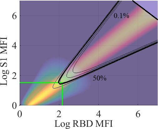
2 of 21                                                 P. N. Patrone & A. J. Kearsley

     To address this problem, we develop a hierarchy of classification strategies that leverage optimal de-
cision theory to maximize both sensitivity and specificity under different real-world conditions (Berger
(1985)). Moreover, our method works for data of arbitrary dimension, e.g. simultaneous measurements
of distinct SARS-CoV-2 antibodies. The simplest form of our analysis uses continuous probability mod-
els and an assumed prevalence to define a loss function in terms of the false-classification rate of the
assay; optimization thereof yields the desired classification strategy. We next generalize this framework
by allowing for uncertainty in the prevalence as characterized by a range of admissible values. This
motivates a modification of the loss function that leads to a third class of indeterminate or “hold-out”
samples that are at high risk of false classification. These hold-outs are candidates for further investi-
gation. In the event that additional testing is unavailable or inconclusive, we develop an algorithm that
leverages information about existing measurements to estimate the prevalence and subsequently deter-
mine the optimal classification strategy. We demonstrate the usefulness of this analysis for a recently
developed SARS-CoV-2 antibody assay (Liu et al. (2020)), provide corresponding proofs of optimality,
and present numerical results validating our results.1
     A key motivation for our work is the fact that many serology tests define positive samples to be those
falling outside the 3σ confidence intervals for negatives (Algaissi et al. (2020), Grzelak et al. (2020),
Hachim et al. (2020), Jacobson (1998)). Since one population does not generally contain information
about another, this assumption yields logical misconceptions. Moreover, 3σ confidence intervals are
only guaranteed to bound roughly 88% of measurements, not 99.7% as is sometimes assumed in liter-
ature (Tchebichef (1867)).2 This consideration is especially important for heavy tailed and/or bimodal
distributions, which may occur in biological settings (Jacobson (1998)). Inattention to such details can
therefore introduce unnecessary inaccuracy in testing.
     Our work addresses such issues by leveraging the idea that mathematical modeling can and should be
be built into all steps of the analysis. This manifests most clearly in the formulation of our loss function,
which is expressed explicitly in terms of probability density functions (PDFs) that characterize training
data. As a natural extension, we also discuss how sources of measurement uncertainty (e.g. arising
from the properties of photodetectors in fluorescence measurements) contribute to these models. This
thorough attention to the underlying physics and behavior of the data is necessary to fully extract the
information contained in measurements and permits us to quantify additional errors induced by simpler
approaches based on thresholds.
     A limitation of our approach is that we cannot fully remove subjectivity of the modeling.3 In par-
ticular, limited training data leads to situations in which we must empirically determine parameterized
distributions of measurement outcomes associated with positive or negative samples. However, this
problem diminishes with increasing amounts of data and, in the case of testing at a nation-wide scale,
likely becomes negligible (Patrone & Rosch (2017)); see Seronet operations for examples of such test-
ing at scale (NCI (2021)).4 Moreover, all classification schemes contain subjective elements, so that our
   1 Certain commercial equipment, instruments, software, or materials are identified in this paper in order to specify the ex-

perimental procedure adequately. Such identification is not intended to imply recommendation or endorsement by the National
Institute of Standards and Technology, nor is it intended to imply that the materials or equipment identified are necessarily the
best available for the purpose.
   2 This observation is a direct consequence of the Chebyshev inequality.
   3 While subjectivity is often not bad per-se, the context of serology testing for a disease such as COVID-19 requires special

consideration: (i) serology testing is used to inform large-scale healthcare policy decisions; and (ii) it is reasonable to assume that
there is an objective (but potentially unknown) truth as to whether an individual has been previously infected. Clearly, there is
significant motivation to uncover this objective truth. We take the perspective that classification is improved through modeling
that reflects as much as possible the objectivity of the underlying phenomena.
   4 In particular, large amounts of empirical data can be used to accurately reproduce probability density functions using spectral
Classification under Uncertainty 3 of 21
analysis is not unique in this regard. In contrast, we explicitly highlight elements of our approach that
are candidates for revision and point to open directions in modeling.
We also note that our analysis is related to likelihood classification, which has seen a variety of
manifestations in the biostatistics community; see, for example, works on receiver operating character-
istics (ROC) (Florkowski (2008)). However, we show that these methods are special cases of a more
general (and thus more powerful) framework that leverages conditional probability to directly reveal the
role of disease prevalence on the classification problem. This generality also provides the mathematical
machinery needed to account for uncertainty in the prevalence and demonstrate how it impacts classifi-
cation. In the Discussion section we revisit these comparisons in more detail and frame our work in a
larger historical context.
The remainder of the manuscript is organized as follows. Section 2 reviews key notation. Section
3 develops the theory behind our hierarchy of classification strategies. Section 4 illustrates the imple-
mentation of these strategies for a SARS-CoV-2 antibody assay developed in Ref. (Liu et al. (2020)).
Section 5 provides numerical results that demonstrate optimality and statistical properties of our classi-
fication strategy. Section 6 provides more context for and discussion of our work. Proofs of key results
are provided in an appendix.
2. Notation and Terminology
Our analysis makes heavy use of set and measure theory. In this brief section, we review key notation
and ideas. Readers familiar with set theory and classification problems may skip this section.
• By a set, we mean a collection of objects, e.g. measurements or measurement values.
• The symbol ∈ indicates set inclusion. That is, r ∈ A means that r is in set A.
• The symbol 0/ denotes the empty set, which has no elements.
• The operator ∪ denotes the union of two sets. That is, C = A ∪ B is the set containing all elements
that appear in either A or B.
• The operator ∩ denotes the intersection of two sets. That is, C = A ∩ B is the set of elements
shared by both A and B.
• The operator / denotes the set difference. We write C = A/B to mean the set of all objects in A
that are not also in B. Note that in general, A/B 6= B/A.
• The notation A = {r : ∗} defines the set A as the collection of r satisfying condition ∗.
Throughout, we frequently refer to two types of data: (i) training data, for which the underlying
class is known a priori; and (ii) test data, which is assumed to have an unknown class and is the data to
which a classification method is ultimately applied.
3. Decision-Theory Classification Framework
Our classification framework begins by assuming that each patient or sample can be associated with a
measurement value r in some set Ω ⊂ RN . The elements of r represent, for example, the fluorescence
methods; see, e.g. Ref. (Patrone & Rosch (2017)).4 of 21 P. N. Patrone & A. J. Kearsley
intensities of different colors recorded by a photodetector, where the light is assumed to be emitted by
fluorophores attached to SARS-CoV-2 antibodies. In the examples that follow in Sec. 4, we take r to be
a two-dimensional vector whose entries are the amount of fluorescent light presumably associated with
receptor binding-domain (RBD) and spike (S1) antibodies for SARS-CoV-2. It is noteworthy that even
for samples with no known SARS-CoV-2 antibodies, it is possible for instruments to record non-zero
signals associated with non-specific binding of fluorophores to other biological molecules in the sample,
for example; see Fig. 1 and Ref. (Liu et al. (2020)).
In this context, we assume that there are two populations, one corresponding to patients who have
had COVID-19 (whether confirmed or not), and the other corresponding to individuals who have not
been infected. Furthermore, we assume that the conditional probability densities of measurement out-
comes r for these populations are P(r) and N(r). That is,
P : Ω 7→ R (1)
yields the probability of a measurement value r for a known positive sample, and N(r) likewise yields
the corresponding probability for a known negative sample.
In general, construction of the conditional PDFs P(r) and N(r) requires training data whose classes
have been confirmed by another measurement technique. In the case of SARS-CoV-2 testing, positive
training samples are taken from patients who have previously tested positive via quantitative polymerase
chain-reaction (qPCR) measurements, whereas negative samples are known to have been drawn before
the pandemic; see Ref. (Liu et al. (2020)). In Sec. 4 we further consider construction of these conditional
PDFs. In this section, we assume that these functions are given. Figure 1 shows an example of training
data first reported in Ref. (Liu et al. (2020)). Moreover, unless otherwise specified, we assume in this
section that r corresponds to a test data-point.
If 0 6 p 6 1 denotes disease prevalence, then the probability density Q(r) of a measurement r for
an unclassified sample is given by
Q(r) = (1 − p)N(r) + pP(r). (2)
The interpretation of Eq. (2) is straightforward. The first term on the right-hand side (RHS) is the
probability that the sample is negative times the probability density that a negative sample has value r,
while the second term bears the corresponding interpretation for positive samples. It is straightforward
to verify that Q(r) so defined is normalized provided this condition holds for the conditional PDFs.
Given Eq. (2), the goal of our classification framework is to define an appropriate pair of domains
D?P and D?N such that we classify test data r ∈ D?P and r0 ∈ D?N as positive and negative, respectively. To
achieve this, we pursue an approach motivated by likelihood ratios; see, e.g. Ref (Berger (1985)). We
first consider arbitrary partitions DP and DN (corresponding to positive and negative classes) and seek
to define a “classification error” in terms of them. Intuitively, we require that the DN and DP have the
properties that:
DP ∩ DN = 0,
/ (3)
i.e. a point is either positive or negative, but not both; and
DP ∪ DN = Ω , (4)
i.e. any measurement can be classified.Classification under Uncertainty 5 of 21
FIG. 1. Training data from an Immunoglobulin G (IgG) serology test described in Ref. (Liu et al. (2020)). Red × and blue o
correspond to known positives and negatives. The steps for constructing the scaled receptor binding-domain (RBD) and spike
(S1) mean-fluorescence intensity (MFI) values are described in the first two paragraphs of Sec. 4, where they are denoted x and
y, respectively. Colored domains correspond to a hypothetical binary classification scheme for identifying samples as negative
(teal) or positive (yellow). The green boundary separating the domains is a 3σ confidence interval estimated in Sec. 4. If we
treat the training data as test data, the classification scheme based on cofidence intervals incorrectly classifies some positive and
negative samples.
Within this general setting, we define the classification error for test data to be the loss function
Z Z
Lb [DP ,DN ] = (1− p) dr N(r)+ p dr P(r). (5)
DP DN
The two terms on the RHS of Eq. (5) are the average rates of false positives and negatives as a function
of the DN and DP . In practical applications we want the smallest error rate possible; thus, we define the
optimal domains D?N and D?P to be those that minimize Lb . We remind the reader that in this formulation,
p, P(r), and N(r) are assumed to be known. We revisit this point below.
From a mathematical standpoint, however, we immediately encounter an annoying technical detail
that requires attention. Specifically, any set X whose probabilities
Z Z
µP (X) = dr P(r) = dr N(r) = µN (X) = 0 (6)
X X
are zero can be assigned to either DP or DN without changing Eq. (5). In particular, we may move any
individual point r0 or discrete collection thereof between sets if P(r) and N(r) are bounded.5 Thus, it
is clear that the optimization problem given by Eq. (5) subject to constraints (3) and (4) does not have a
unique solution.
The resolution to this problem is to recognize that any DN and DN 0 differing by sets X of probability
or measure zero are, for all practical purposes, the same. Thus, we weaken the constraints (3) and (4) to
Z
5 The probability of an event associated with measurement r is given by lim Q(r) dr , where B(r, ε) is a ball centered at r
ε→0 B(r,ε)
having radius ε. Provided that Q(r) is sufficiently smooth in the vicinity of r, this integral converges to zero.6 of 21 P. N. Patrone & A. J. Kearsley
only require that
µP (DN ∩ DP ) = µN (DN ∩ DP ) = 0 (7a)
µP (DN ∪ DP ) = µN (DN ∪ DP ) = 1 (7b)
and treat all sets DN and DN 0 as being equivalent if µN (DN ) = µN (DN 0 ) and µP (DN ) = µP (DN 0 ), etc.6
The value of unity appearing on the RHS of Eq. (7b) is the probability of any event happening, which is
distribution independent.
With these observations in mind, it is straightforward to show [see Appendix A] that under physically
reasonable conditions (e.g. bounded PDFs), the domains
D?P = {r : pP(r) > (1 − p)N(r)} (8)
D?N = {r : (1 − p)N(r) > pP(r)} (9)
(or any sets differing by measure zero) minimize Lb subject to the constraints (7a) and (7b). It is notable
that the prevalence p enters the definitions in Eqs. (8) and (9). We recognize this as a manifestation of the
observation mentioned in the introduction: the optimal classification strategy depends on the prevalence.
For example, if p = 0, the set D?P = 0, / which is the obvious conclusion that one should never classify
any samples as positive if there is no disease. Conversely, when p = 1, D?N = 0, / i.e. one should never
classify a sample as negative. Thus, for intermediate values of prevalence, the sets defined by Eqs. (8)
and (9) provide an optimal interpolation between these degenerate cases.
From a diagnostic perspective, Eqs. (5)–(9) are problematic in that p is often unknown a priori. In
fact, estimates of p are often the target of a widespread testing study. Moreover, the data used to estimate
p may not characterize different populations to which the test is later applied, and/or models of P(r) and
N(r) may be biased. Such problems are likely to be especially pronounced at the onset of a pandemic,
when prevalence of a disease has large geographic variation and/or available data heavily reflects small
sub-populations.
To address this problem, we propose that the prevalence be specified only up to some interval, i.e.
pl 6 p 6 ph for two constants pl , ph . This uncertainty in the prevalence can simultaneously account for
effects such as lack of sufficient data and/or geographic variability in the diseases. Appropriate choices
for pl and ph are problem specific.
A side-effect of permitting p to be uncertain is that the binary classification scheme induced by Eq.
(5) is no longer well-posed. For example, it is obvious that the sets
D?p (pl ) = {r : pl P(r) > (1 − pl )N(r)} 6= {r : ph P(r) > (1 − ph )N(r)} = D?p (ph )
are not equivalent if they differ by more than a set of measure zero. Thus, minimizing Lb does not define
unambiguous, optimal classification domains. A solution is to recognize that uncertainty in prevalence
leads to a third class for which we cannot make a meaningful decision without further information. This
motivates us to set-aside constraints (7a) and (7b).
In their absence, however, the loss function given by Eq. (5) develops a degenerate solution. Specif-
ically, it is minimized by setting DN = DP = 0, / which yields Lb [0, / = 0. In other words, we minimize
/ 0]
false results by never making a decision. Since this degenerate solution is not useful, we consider a
6 In mathematical language, we consider equivalence classes of sets defined up to sets of measure zero.Classification under Uncertainty 7 of 21
ternary loss function given by
Z Z
Lt [D p , DN ] = (1 − pl ) dr N(r) + ph dr P(r)
DP DN
Z Z
− pl dr P(r) − (1 − ph ) dr N(r). (10)
DP DN
Equation (10) computes worst-case averages of false (top line) and correct (bottom line) classification;
moreover, −1 6 Lt 6 1. Choosing to not make a decision has the effect of decreasing the first two
terms while increasing the last two. Thus, minimizing Eq. (10) with respect to the DP and DN balances
holding-out samples with the loss of accuracy in correctly classifying measurements.
While technical details are reserved for Appendix A, it is straightforward to show that (up to sets of
measure zero) Lt is minimized by the sets
D?P = {r : pl P(r) > (1 − pl )N(r)} (11)
D?N = {r : (1 − ph )N(r) > ph P(r)}. (12)
The set H of samples to hold out is given by the set difference H = Ω / (D?N ∪ D?P ).
When the “hold-out” class H does not represent a viable end-point characterization of a sample,
there are several follow-up strategies. For example, one can perform additional tests that may be more
sensitive and/or provide additional information with which to make a decision. A second approach is to
combine several measurements to estimate a “pooled” prevalence p̂ associated with the corresponding
sub-population. To understand how this method works, consider an arbitrary partition DN and DP .
Define
Z
QP = dr Q(r) = p̂Pp + (1 − p̂)N p (13)
DP
R R
where Pp = DPdr P(r) and N p = DPdr N(r) are known and p̂ is the unknown pooled prevalence. Also
construct the estimator
1 S
QP ≈ Q̄P = ∑ I[ri ∈ DP ], (14)
S i=1
where I[ri ∈ DP ] is the indicator function that the ith sample ri is in DP and S is the total number of
samples. Combining Eqs. (13) and (14) yields
QP − NP Q̄P − NP
p̂ = ≈ . (15)
Pp − N p Pp − N p
This estimate can then be used in place of p appearing in the loss function Lb , leading to corresponding
definitions of D?P and D?N according to Eqs. (8) and (9).
A few comments are in order. The interpretation of Eq. (15) follows from the recognition that Pp and
N p are the rates of true and false positives in DP when p = 1 and p = 0, respectively. Thus, when the
empirical rate of positives approaches N p , all of the positives are due to false negatives, and prevalence
is zero. Conversely, when Q̄P → PP , the positives arise entirely from true positives, so that p = 1.
Moreover, when the PDFs P(r) and N(r) are known, the prevalence estimate p̂ is unbiased, meaning
that its average value equals the true prevalence. This is a direct consequence of the fact that Q̄P is a
Monte Carlo estimate of the integral defining QP . For the same reason, p̂ also converges to p in a mean-
squared sense when the number of samples S → ∞. The convergence rate is known to decay as S−1/2
(Caflisch (1998)). Thus, we anticipate that errors in the estimates of the optimal domains are likewise
bounded; see also Sec. 5.8 of 21 P. N. Patrone & A. J. Kearsley
FIG. 2. Training data from Ref. (Liu et al. (2020)) and conditional probability models thereof. The red × and blue o are known
positives and negatives. The horizontal axis displays the logarithm of normalized mean-fluorescence intensity (MFI) measure-
ments for the RBD antibodies. The vertical axis corresponds to the S1 antibodies. Contour lines describe the PDFs associated
with positive (gold) and negative populations (teal) according to Eqs. (16) and (17). The
4. Example Applied to SARS-CoV-2 Antibody Data
To illustrate the ideas of the previous section, we consider data associated with a SARS-CoV-2 assay
developed in Ref. (Liu et al. (2020)). In that work, the authors generated a set of training data, which
we use to construct our conditional probability models. As suggested in Sec. 3, positive training data
came from individuals who had previously been confirmed (via qPCR) to have contracted SARS-CoV-
2, while negative data is associated with samples that were collected before emergence of the virus. In
Figs. 1–4, the positive and negative training data correspond to red × and blue o. The original files
containing raw data are supplied with the supplemental information in Ref. (Liu et al. (2020)).
To construct P(r) and N(r), we consider the first 418 Immunoglobulin G (IgG) samples as candidate
training data. For each sample, we use both the MFI values associated with the RBD and S1 protein.
For positive samples, we further restrict attention to those for which symptoms began at least 7 days
before the test. We reject any samples in which the raw MFI is less than -300, as this may correspond to
a significant instrument calibration artifact that biases results. This leaves a total of 58 positive and 343
negative samples for use as our final training data set.
As a preliminary step, we observe that the MFI values range from roughly -300 to 6.3 × 10⁴ . More-
over, many of the IgG data fall on top of one another at this upper limit, which would happen if the
signals saturated the photodetector. These observations are thus consistent with the data being recorded
by a signed, 16-bit digitizer.7 We speculate that the negative MFI values are due to dark currents and/or
small voltage offsets inherent in photodetector equipment. To approximately account for such effects,
7 The digitizer may be 20 bits or more, since several levels of decimal accuracy are also specified.Classification under Uncertainty 9 of 21 FIG. 3. Sample SARS-CoV-2 IgG antibody training data from Ref. (Liu et al. (2020)) and classification domains obtained by minimizing Eq. (5) with p = 58/401, the true prevalence of this set. The red × and blue o are known positives and negatives. The horizontal axis displays the logarithm of normalized mean-fluorescence intensity (MFI) measurements for the RBD antibodies. The vertical axis corresponds to the S1 antibodies. The green lines are the sample mean plus 3σ confidence intervals for negative samples, commonly used as the basis for classification of positive samples. The negative classification domain D?N is purple, whereas the positive classification domain D?P is yellow. The calculated error rate (sum of rates of false negatives and false positives) for the optimal classification strategy (blue and yellow domains) is 2.24%, whereas the error rate for the 3σ classification scheme (box bounded by green lines) is 3.74%. FIG. 4. Training data and classification domains according to optimization of Eq. (10) for pl = 0.01 and ph = 0.9. Data and color schemes are the same as for Fig. 3. Note that the hold-out (teal) region between positive and negative regions contains both positive and negative training samples that are close together, consistent with the recognition that these would be high-risk for mis-classification were they test data.
10 of 21                                     P. N. Patrone & A. J. Kearsley

we add 300 units to all measured values. To adjust for variable geometric factors, we normalize the raw
MFI data by a reference signal, as indicated in Liu et al. (2020); see also the supplemental data files in
that reference for more details. To set a relative scale for the data, we then divide by smallest MFI value
separately for RBD and S1. We denote the corresponding measurements by x (RBD) and y (S1). For
clarity of notation, we denote this pair of values as r = (x, y) (as opposed to r, which is reserved for
later use).
    Figure 1 shows the training data r, which spans several decades; it is useful to work with its log-
arithm. This transformation: (i) ensures that the negative populations are near the origin and in the
upper-right quadrant; and (ii) better separates measurements at the boundary of negative and positive
populations. We denote points in this space by r = (x, y) = log(r) = (log[x], log[y]) and work directly
with the r.
    To construct the conditional PDF for negative populations, we first note that there is likely to be a
small amount non-specific signal due to other antibodies, e.g. associated with different coronaviruses;
see Ref. (FDA (2020)) and the documents therein. Moreover, we observe that the RBD is a substructure
of the S1 protein (Walls et al. (2020)). Thus, it is plausible that antibodies that can bind to RBD will
also be detected in an S1 assay (Tian et al. (2020)); i.e. their signals should
                                                                            √ be correlated√for any given
sample. This motivates a change of variables of the form z = (x + y)/ 2, w = (x − y)/ 2, where we
expect probability mass to be concentrated along the line w = 0. We next postulate a hybrid gamma-
Gaussian distribution of the form
                                                                              2
                                         zk−1       −z−z−
                                                            (w−µ)
                               N(r) = √            e θ β 2α 2 exp(2z/β ) ,                            (16)
                                       2παΓ (k)θ k
where θ , k, α, µ, and β are parameters to be determined. The Gaussian term depending on w in Eq.
(16) enforces the desired correlation between S1 and RBD measurements, while the gamma distribution
in z is an empirical choice that allows for a long tail from the origin. We estimate the model parameters
using a maximum likelihood estimate (MLE). For simplicity, we subsequently restrict the PDFs to the
domain 0 6 x, y 6 7. This cuts off roughly 0.5% of the probability mass associated with the model, so
that we renormalize Eq. (16) to this domain. See Fig. 2.
    Given that the positive measurements span roughly the entire line x = y, we model them via a hybrid
beta-Gaussian distribution of the form
                                                                                  2
                                               ζ α−1 (1−ζ )β −1 − (w−µ)
                             P(r) = Γ (α +β ) p                   e 2θ 2 ζ                          (17)
                                              θ 2πζ Γ (α)Γ (β )
                      √                    √
where ζ = (x + y)/(9 2) and w = (x − y)/ 2. The parameters α, β , θ , and µ are determined by MLE.
As before, the transformed coordinates and Gaussian on w enforce the expected correlation structure
between S1 and RBD signals. The factor of 9 in the definition
                                                    √          of ζ is a modeling choice of an approxi-
mate upper bound on the measured values of (x + y)/ 2 and rescales the beta distribution to its standard
domain of 0 6 ζ 6 1. The use of this PDF is consistent with the observation that the digitizer enforces
upper and lower limits on the MFI that are reported by the instrument. As for N(r), we restrict Eq. (17)
to the domain 0 6 x, y 6 7 and renormalize the PDF to have unit probability. See Fig. 2.

    Finally, we note the probability densities P(r) and N(r) can be expressed in the original units, e.g.
via transformations of the form
                                                            1
                                        P(r) = P(log(r))      .                                     (18)
                                                          xy
Classification under Uncertainty 11 of 21
FIG. 5. Evaluation of Lb as a function of the assumed prevalence p̃ defining the domain of positive and negative classification; see
Eqs. (20) and (21). The true prevalence for each curve is denoted by p. The false negatives and positives for a given prevalence
are indicated by dotted lines. The minmum error is obtained when the assumed prevalence p̃ equals the true prevalence, i.e. p̃ = p.
In practical applications, it is also useful to define a likelihood ratio R(r)
P(r)
R(r) = , (19)
N(r)
whenever N(r) 6= 0 over the domain for which P(r) 6= 0. While not strictly necessary, the likelihood
ratio simplifies the definitions of D?N and D?P .
Figure 3 illustrates the classification strategy according to Eqs. (8) and (9), which minimize Eq.
(5). As an initial validation, we apply our analysis to the training data as if it were test data. We set
p = 58/401, which is the true prevalence for this example. The negative domain D?N is purple, whereas
the positive domain D?P is yellow. We also plot the mean plus 3σ confidence intervals (green lines)
associated with the negative MFI measurements, which are often used to define classification domains;
see also Ref. (JCGM (2008)). Several of the negative samples fall beyond this boundary and would
thus be characterized incorrectly, while our optimization-based method correctly classifies all but one.
Moreover, our approach correctly identifies 50 of 58 positives, whereas the original method discussed
in Liu et al. (2020) was only correct in 45 of 58 cases.
Figure 4 shows the corresponding results for the domains defined by Eqs. (11) and (12), with pl =
0.01 6 p 6 0.9 = ph . Colored domains have the same meanings as in Fig. 3. While the majority of
samples are classified as in Fig. 3, a small hold-out region (teal) has opened up between D?N and D?P .
This region contains both positive and negative samples, consistent with the observation that they are
high-risk for mis-classification. It is interesting to note, however, that the new part of the holdout region
is small compared to D?P and D?N , despite the uncertainty in the prevalence being so high.12 of 21 P. N. Patrone & A. J. Kearsley
FIG. 6. Plot of boundaries defining candidate domains DP ( p̃) as a function of presumed prevalence p̃ [see Eq. (20)]. The contour
labels correspond to 50%, 14.46% (bold), 10%, 1%, and 0.1% prevalence. The colormap is the superposition of P(r) and N(r)
weighted according to p; see also Fig. 2. For a given contour, all measurement values inside and to the right of the contour would
be classified as positive for that domain D p ( p̃), whereas all values to the left would be negative. The green box corresponds to
the mean plus 3σ LOD, while the bold black contour is the boundary between optimal classification domains. Note that if the
samples inside the green box were classified negative and all others positive, the classification scheme would lead to additional
false negatives.
5. Computational Validation
The example in the previous section illustrate a range of issues that must be considered in estimating the
probability densities P(r) and N(r). Our goal in this section is to numerically demonstrate the sense in
which the classification strategies presented above are optimal. In the following examples, we use the
same PDFs as constructed in the previous section.
As a first test, we numerically compute the loss function given by Eq. (5) for three difference preva-
lence values (p = 1/10, p = 1/5, and p = 1/2) over the domains
D p ( p̃) = {r : R(r) > p̃/(1 − p̃)} (20)
Dn ( p̃) = {r : R(r) < (1 − p̃)/ p̃} (21)
for p̃ ranging from 0.01 to 0.9. Note that p̃, which is distinct from the true prevalence p, is an assumed
prevalence required to define trial classification domains. As expected, the minimum error (sum of
false negatives and false positives) is obtained when p̃ = p, consistent with Eqs. (8) and (9). It is also
interesting that the error increases rapidly with increasing p̃ in the vicinity of p̃ = 1. Physically, this
arises from the fact that p̃ = 1 assumes a prevalence of 100%, for which all of the samples would
be classified as positive. In this limit, the error is Lb = 1 − p, since all of the negative samples are
incorrectly classified. Corresponding statements hold for the limit p̃ = 0.
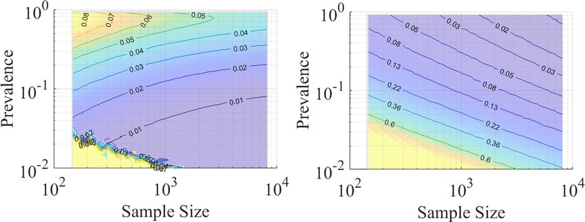
Figure 6 highlights these observations in more detail. The colormap is the superposition of P(r)Classification under Uncertainty 13 of 21 FIG. 7. Total error rates (false positives plus false negatives) and standard deviations for different sample sizes and prevalence values. Left: Mean error plus 3 standard deviations (contour lines) of the error as a function of sample size and prevalence, computed over 10,000 realizations of samples for each prevalence-sample-size pair. Right: Standard deviation of the error as a function of sample size for fixed prevalence values ranging from roughly p = 0.9 (top line) to p = 0.005 (bottom line). FIG. 8. Adaptive routine to approximate optimal classification for prevalence of p = 1/10001, which is initially unknown to the algorithm. We generate 106 synthetic negative measurements (blue o) and 100 synthetic positive measurements (red ×); see main text for details. The shaded regions correspond to classification domains DP and DN as a function of the algorithm iteration. We set the initial classification domains DN (purple) and DP (union of teal and yellow) to correspond to a prevalence of 50% and use the Eq. (15) to estimate a new prevalence. This yields updated positive (yellow) and negative domains (union of purple and teal). The fraction of false positives is significantly reduced.
14 of 21                                               P. N. Patrone & A. J. Kearsley

FIG. 9. Error rates in our adaptive algorithm. Left: Average classification error rates as a function of prevalence and sample size.
Right: Mean plus 3-sigma confidence interval for the prevalence error rate. The procedures for generating samples are the same
as in Fig. 7. Note, however, that the prevalence is initially unknown and determined adaptively via Eq. (15), using non-optimal
Dn and D p corresonding to a 50% prevalence.

and N(r) weighted by p = 58/401. The contour lines are boundaries between candidate domains D p (q)
according to Eq. (20), while the black solid line is the optimal boundary separating the negative and
positive classification domains. The green box is the negative population as defined alternatively by the
3σ classification scheme. Note that a significant fraction of the negatives fall outside of that boundary
and would thus be classified incorrectly as positives. Moreover, increasing p̃ forces the positive domain
deeper into the PDF associated with negative samples, increasing the error rate. In the limit p̃ → 1,
DP ( p̃) would entirely cover the plot, although the transition happens rapidly near p̃ = 1 given the shape
of P(r).
    We next test our classification approach in the more realistic scenario of finite data. This illus-
trates the extent to which errors approach their ideal limits and allows us to characterize uncertainty in
prevalence estimates obtained from Eq. (15). We use a random number generator to create M synthetic
measurements according probability distributions used in Figs. 2, where M ranges from 100 to 2 × 10⁶ .
    Figure 7 illustrates the statistical behavior of such tests under the assumption that the prevalence,
and thus the optimal classification domains, are known. We consider 33 sample sizes ranging from
roughly 100 samples to 10,000 samples and 99 prevalence values ranging from roughly 0.005 to 0.9. For
each prevalence-sample-size pair we generate corresponding positive and negative samples, which we
classify using our optimal domains. We compute the total error rate (false positives plus false negatives)
and repeat this exercise 10,000 times. The left plot shows the average error rate plus 3 times the standard
deviation of the error. The right plot shows the standard deviation of the error as a function of sample
size for fixed prevalence values. The decay rate is proportional to inverse-root sample size, which is
consistent with statistical estimators of this type. From the scale of the standard deviation, we see that
total error rate is dominated by its average (i.e. optimal) behavior for as few as 1000 samples, which is
easily achievable in real-world settings.
    Figure 8 illustrates the behavior of our adaptive algorithm under the assumption that the prevalence
is initially unknown to the analysis. This test is representative of how our analysis might be used in
a widespread testing operation in which follow-up is not possible. We set p = 1/10001 and generate
1000100 synthetic samples. The figure demonstrates that when even when the prevalence is initially
unknown, the adaptive algorithm given by Eq. (15) only yields on the order of 15 false negatives and
Classification under Uncertainty 15 of 21
few (if any) false positives. Moreover, in this particular example, the prevalence is estimated to within
1% relative error in terms of p̂, although the characteristic value ranges over roughly 40% with repeat
realizations. Importantly, this estimate is based on Eq. (15) and not the number of samples classified
as positives. The latter are biased low in, since otherwise the number of false positives would rapidly
increase; see also Fig. 6 and discussion thereof.
Figure 9 illustrates further statistical properties of the adaptive algorithm. We consider the same
set of prevalence values and sample sizes as in Fig. 7. The left plot shows that, with the exception of
both low-prevalence and small samples, the mean plus three-sigma estimate of the error rate are approx-
imately the same as for the idealized case in Fig. 7. Thus, the classification rate is not substantively
affected by the unknown prevalence. The right plot shows the mean error in the prevalence plus 3 stan-
dard deviations as computed by Eq. (15). Note that even with this conservative estimate, the relative
error in the prevalence is less than or equal to 20% at a sample size of 1000 tests and true prevalence
of 1/100. Moreover, this estimate rapidly decreases with increasing prevalence and/or sample size. At
a prevalence of 1/10, the relative error in estimated prevalence is only 6% at a sample size of roughly
100. This suggests that the adaptive algorithm may be both robust and accurate in real-world settings.
6. Discussion, Extensions, and Open Questions
6.1 Comparison with Other Classification Strategies
While several classification strategies have been formulated and studied in the context of diagnostic set-
tings (Lo et al. (2014), Jacobson (1998), Florkowski (2008)), we are unaware of a previously developed
mathematical framework that unifies them all. The present discussion illustrates how Eqs. (2), (5), (10),
and extensions thereof address this issue.
For assays that return a scalar measurement, ROC has become a popular method for determining
an “optimal cutoff value” (i.e. a point) separating negative and positive populations. Loosely speaking,
the objective of this method is to select a cutoff that simultaneously maximizes true positives while
minimizing false positives. Because the classification is binary, this is equivalent to minimizing Eq.
(5);8 however, the analysis is typically applied to raw data that has a random, unspecified prevalence.
Thus, the optimization problem being solved is not fully explicit, so that the cutoff may be entirely
unrepresentative of the target population of interest. Moreover, ROC makes an implicit assumption that
the rate of true positives is a one-dimensional (1D) function of false negatives. As this does not hold for
vector r, there is no obvious extension of ROC per se to more complicated measurement settings.
Our formulation in terms of Eq. (5) directly addresses these shortcomings. In particular, the analysis
holds for r of any dimension, since the main results are defined in terms of set theory. Moreover,
the prevalence p appears explicitly in our loss functions. Additionally, in 1D settings, our analysis
reverts to identifying a point r satisfying the equation pP(r) = (1 − p)N(r), which is the same as the
result obtained from ROC were the prevalence explicitly stated. Thus, we see immediately that Eq.
(5) is the generalization of ROC to arbitrary dimensions and prevalence. The benefit of couching the
analysis in terms of loss functions is that one can immediately extend it to more complicated scenarios,
e.g. uncertain prevalence values; see Eq. (10). Just as importantly, we make explicit the modeling
assumptions underlying classification.
As an alternative to overcoming the limitations of ROC, several groups have developed strategies
8 The rate T of true positives is related to false negative F via F = 1 − T . Thus, maximizing true positives is equivalent
p n n p
to minimizing false negatives. For comparison, our analysis minimizes the prevalence-weighted rate of false positives and false
negatives, thereby establishing the stated equivalence.16 of 21 P. N. Patrone & A. J. Kearsley
wherein they use 3σ -type cutoffs in the hopes that this provides a 99% confidence interval (Klumpp-
Thomas et al. (2020), Algaissi et al. (2020), Grzelak et al. (2020), Hachim et al. (2020)). Notably,
such approaches are straightforward to generalize to higher dimensional measurements being used for
SARS-CoV-2 antibody detection. However, the optimal decision-theory framework immediately reveals
that such choices are by construction sub-optimal. Two observations inform this conclusion. First, such
formulations assume that the negative population is well-described by a Gaussian distribution, which
is unreasonable in many biological systems; in other words, the modeling aspect of classification is
overlooked. Second, confidence-interval approaches ignore the dependence of optimal classification on
the prevalence, which controls the impact of overlapping conditional probability distributions. See, for
example, Figs. 6 and 8.
These examples highlight the conclusion that classification is fundamentally a task in mathematical
modeling, and optimality cannot be achieved without due consideration of all aspects thereof. As a
corollary, classification is also subjective. The goal then is to formulate better models by explicilty
understanding and characterizing the underlying measurement process more accurately, since this is
the primary mathematical contribution to the classification error. To the extent possible, uncertainty
arising from instrumentation should also be characterized, since such effects contribute to conditional
measurement outcomes.
In this vein, note that Eq. (15) is the most important result of our analysis. By it, we recognize that
all information about both the optimal classification strategy and the true prevalence can be deduced
by knowing the conditional probability densities P(r) and N(r). The importance of this observation
cannot be understated. Irrespective of the classification error, Eq. (15) yields unbiased estimates of the
prevalence, and more testing reduces uncertainty therein. Moreover, much effort within the community
has been devoted to developing concepts such as limits-of-detection, ROC curves, sensitivity, specificity,
etc. Here we demonstrate that all of these concepts are subsumed by a unifying loss-function defined in
terms of conditional probability densities. All of the relevant information needed compute performance
metrics of a diagnostic test can be deduced directly from P(r), N(r).
6.2 Extensions of our analysis
Equations (5) and (10) can easily be generalized to optimize different relative weightings of false neg-
atives and false positives. Extensions of our method can also incorporate measurement uncertainty. To
achieve this, one can model a measured value m as
m = s + ε. (22)
If E(r) and S(r) are the PDFs associated with ε and s, then the probability density Pm for m is
given by
Z
Pm (r) = dr0 S(r0 )E(r − r0 ) (23)
where integration is over the domain of E.
We also note that
6.3 Relevance to Assay Design
During early stages of assay design, experimental parameters such as “optimal” dilution must be fixed.
However, the definition of what constitutes optimal may be vague or even left unspecified. As anClassification under Uncertainty 17 of 21
alternative, we propose using one of the loss functions Lb or Lt defined in Sec. 3. Mathematically we
recognize then that, in addition to the domains D p and Dn , the loss functions depend on some variables
φ , so that we write generically L = L[D p , Dn , p, φ ], where as before, p is the prevalence. The specific
objective to minimize is subject to the needs of the modelers at hand. However, it is straightforward to
extend the optimization to scenarios in which one wishes, for example, to minimize error over multiple
prevalence values simultaneously. Specifically, one might minimize an objective of the form
H(φ ) = ∑ min Lb [D p , Dn , pi , φ ] (24)
pi D p ,Dn
with respect to the experimental parameters φ for a chosen set of pi . More generally, it is possible to
construct functionals of the objectives Lb and Lt that can quantify the relative importance of error at
different prevalence values, thereby making the concept of an optimal assay more precise.
Figure 6 also points to an interesting alternative. When the PDFs associated with positive and neg-
ative samples are well separated, the classification error may be insensitive to the choice of prevalence
when using Eqs. (8) and (9). Concepts such as the Kullback-Leibler (KL) divergence (also known as the
relative entropy) are frequently used to assess degree of overlap between two probability densities. Thus,
an alternative strategy for developing an optimal assay could amount to maximizing the KL divergence
over the set of design parameters φ . We leave such considerations for future work.
6.4 Key Assumptions and Limitations
Our analysis makes several key assumptions that introduce corresponding limitations. In particular, we
require that the probability densities P(r) and N(r) be known. In previous works (Patrone & Rosch
(2017)), we have developed methods for objectively reconstructing PDFs with high-fidelity given many
measurements, as may be available when testing large portions of a population. However, in general (and
especially at the beginning of an emerging outbreak), there may not be sufficient data reconstruct P(r)
and N(r) without empirical assumptions (e.g. fit functions). These introduce additional uncertainty into
the modeling process, which therefore affects classification error. In Sec. 4, these assumptions entered
via our use of the gamma and beta distributions. Moreover, characterizing the conditional PDFs may be
challenging high-dimensional situations, e.g. when 3 or more antibody targets are used for classification.
While beyond the scope of this work, there are several potential strategies to address such short-
comings. In the event that a binary classification is required (e.g. no holdouts), it may be possible to
formulate a parameterized collection of admissible PDFs characterizing the positive population and de-
fine a consensus loss function as an average over the corresponding individual loss functions. Thus, the
error itself becomes a random variable, and one seeks the classification scheme that minimizes the aver-
age error. Equation (28) in the appendix yields the increase in error due to using a sub-optimal domain,
which may be easily adaptable to the situation in which the PDFs are uncertain. If such approaches are
untenable and holdouts are allowed, an alternative is to use uncertainty in the prevalence as a proxy.
Another key assumption of our work is that P(r) is time-independent. In the case of SARS-CoV-
2, however, it is well known that antibody levels decrease in time, sometimes to the point of being
undetectable after a few months (Patel et al. (2020), Ibarrondo et al. (2020)). From a measurement
standpoint, this is challenging because it means that the loss function L is itself also a function of time
by virtue of its dependence on P. To maintain optimal error rates, it is thus necessary to know this time
dependent behavior, which is beyond the scope of this work.
Acknowledgements: This work is a contribution of the National Institute of Standards and Technol-
ogy and is not subject to copyright in the United States. The authors wish to thank Ligia Pinto for useful18 of 21 P. N. Patrone & A. J. Kearsley
discussions during preparation of this manuscript. We also thank Lili Wang for preliminary discussions
that motivated us to define the scope of this work.
Research involving Human Participants and/or Animals: Use of data provided by Liu et al. (2020)
has been reviewed and approved by the NIST Research and Protections Office.
Data Availability: Analysis scripts developed as a part of this work are available upon reasonable
request. Original data is provided in Ref. (Liu et al. (2020)).
A. Derivation of Classification Domains
In this appendix, we demonstrate that the domains defined in Eqs. (8)–(9) and Eqs. (11)–(12) minimize
the loss functions Lb and Lt .
Lemma 1. Let Lb [DP , DN ] be as defined in Eq. (5), and assume that the PDFs P(r) and N(r) are
bounded and summable functions. Then D?P and D?N as defined in Eqs. (8) and (9) minimize Lb up to
sets of measure zero.
Proof: Without loss of generality (but abusing notation slightly), absorb the constants p and n into
P(r) and N(r), so that we may consider the simpler loss function
Z Z
Lb [DP , DN ] = dr N(r) + dr P(r) (25)
DP DN
Consider sets D̂P and D̂N that differ from D?P and D?N by more than a set of measure zero. It is clear that
(in the sense of Lebesgue integrals) we can decompose Lb [D̂P , D̂P ] as
Z Z
Lb [D̂P , D̂N ] = dr N(r) + dr N(r)
D̂P ∩D?P D̂P /D?P
Z Z
+ dr P(r) + dr P(r), (26)
D̂N ∩D?N D̂N /D?N
where / is the set difference operator. Likewise, we can decompose
Z Z
Lb [D?P , D?N ] = dr N(r) + dr N(r)
D̂P ∩D?P D?P /D̂P
Z Z
+ dr P(r) + dr P(r). (27)
D̂N ∩D?N D?N /D̂N
Subtracting Eq. (27) from (26) yields
∆ L = Lb [D̂P , D̂N ] − Lb [D?P , D?N ]
Z Z
= dr N(r) − dr P(r)
D̂P /D?P D?N /D̂N
Z Z
+ dr P(r) − dr N(r). (28)
D̂N /D?N D?P /D̂P
We recognize that up to a set of measure zero (with respect to both P and N), the sets D̂P /D?P and
D?N /D̂N are the same; that is, any measurable set added to D?P to yield D̂P must be taken from D?N toREFERENCES 19 of 21
yield D̂N . Thus, we find
Z
∆L = dr [N(r) − P(r)]
D̂P /D?P
Z
+ dr [P(r) − N(r)] (29)
D̂N /D?N
By definition of D?P and D?N , it is clear that N(r) − P(r) > 0 for r ∈ D̂P /D?P , whereas P(r) − N(r) > 0
for r ∈ D̂N /D?N . Since these are sets of measure greater than zero, we find immediately that ∆ L > 0,
so that D?P and D?N are optimal up to sets of measure zero. Moreover, it is obvious that the result holds
if only one of either D̂N /D?N or D̂P /D?P has measure greater than zero.
The proof of optimality for Eqs. (11) and (12) is similar in spirit.
Lemma 2. Let Lt [DP , DN ] be as defined in Eq. (10), and assume that the PDFs P(r) and N(r) are
bounded and summable functions. Then D?P and D?N as defined in Eqs. (8) and (9) minimize Lb up to
sets of measure zero.
Proof: As before, consider sets D̂P and D̂N that differ from D?P and D?N by more than a set of measure
zero. Define
∆ Lt = Lt [D̂P , D̂N ] − Lt [D?P , D?N ]. (30)
It is straightforward to show that up to sets of measure zero, the difference can be expressed as
Z Z
∆ Lt = dr nh N(r) − pl P(r) + dr pl P(r) − nh N(r)
D̂P /D?P D?P /D̂P
Z Z
+ dr ph P(r) − nl N(r) + dr nl N(r) − ph P(r). (31)
D̂N /D?N D?N /D̂N
From the definitions Eqs. (11) and (12), it is clear that each of these integrals is positive; thus ∆ Lt > 0.
Moreover, this result holds if any one of the set differences has non-zero measure. .
References
Algaissi, A., Alfaleh, M. A., Hala, S., Abujamel, T. S., Alamri, S. S., Almahboub, S. A., Alluhaybi,
K. A., Hobani, H. I., Alsulaiman, R. M., AlHarbi, R. H., ElAssouli, M.-Z., Alhabbab, R. Y., Al-
Saieedi, A. A., Abdulaal, W. H., Al-Somali, A. A., Alofi, F. S., Khogeer, A. A., Alkayyal, A. A.,
Mahmoud, A. B., Almontashiri, N. A. M., Pain, A. & Hashem, A. M. (2020), ‘Sars-cov-2 s1 and
n-based serological assays reveal rapid seroconversion and induction of specific antibody response in
covid-19 patients’, Scientific Reports 10(1), 16561.
Berger, J. (1985), Statistical Decision Theory and Bayesian Analysis, Springer Series in Statistics,
Springer.
Bermingham, W. H., Wilding, T., Beck, S. & Huissoon, A. (2020), ‘Sars-cov-2 serology: Test, test, test,
but interpret with caution!’, Clinical Medicine 20(4), 365–368.
Bond, K., Nicholson, S., Lim, S. M., Karapanagiotidis, T., Williams, E., Johnson, D., Hoang, T., Sia,
C., Purcell, D., Mordant, F., Lewin, S. R., Catton, M., Subbarao, K., Howden, B. P. & Williamson,
D. A. (2020), ‘Evaluation of Serological Tests for SARS-CoV-2: Implications for Serology Testing
in a Low-Prevalence Setting’, The Journal of Infectious Diseases 222(8), 1280–1288.20 of 21 REFERENCES Caflisch, R. E. (1998), ‘Monte carlo and quasi-monte carlo methods’, Acta Numerica 7, 1–49. FDA (2020), ‘Eua authorized serology test performance’, https://www.fda.gov/medical- devices/coronavirus-disease-2019-covid-19-emergency-use-authorizations-medical-devices/eua- authorized-serology-test-performance. Accessed: 2020-09-16. Florkowski, C. M. (2008), ‘Sensitivity, specificity, receiver-operating characteristic (roc) curves and likelihood ratios: communicating the performance of diagnostic tests’, The Clinical biochemist. Re- views 29 Suppl 1(Suppl 1), S83–S87. Grzelak, L., Temmam, S., Planchais, C., Demeret, C., Tondeur, L., Huon, C., Guivel-Benhassine, F., Staropoli, I., Chazal, M., Dufloo, J., Planas, D., Buchrieser, J., Rajah, M. M., Robinot, R., Porrot, F., Albert, M., Chen, K.-Y., Crescenzo-Chaigne, B., Donati, F., Anna, F., Souque, P., Gransagne, M., Bel- lalou, J., Nowakowski, M., Backovic, M., Bouadma, L., Le Fevre, L., Le Hingrat, Q., Descamps, D., Pourbaix, A., Laouénan, C., Ghosn, J., Yazdanpanah, Y., Besombes, C., Jolly, N., Pellerin-Fernandes, S., Cheny, O., Ungeheuer, M.-N., Mellon, G., Morel, P., Rolland, S., Rey, F. A., Behillil, S., Enouf, V., Lemaitre, A., Créach, M.-A., Petres, S., Escriou, N., Charneau, P., Fontanet, A., Hoen, B., Bruel, T., Eloit, M., Mouquet, H., Schwartz, O. & van der Werf, S. (2020), ‘A comparison of four serological assays for detecting anti–sars-cov-2 antibodies in human serum samples from different populations’, 12(559). Hachim, A., Kavian, N., Cohen, C. A., Chin, A. W. H., Chu, D. K. W., Mok, C. K. P., Tsang, O. T. Y., Yeung, Y. C., Perera, R. A. P. M., Poon, L. L. M., Peiris, J. S. M. & Valkenburg, S. A. (2020), ‘Orf8 and orf3b antibodies are accurate serological markers of early and late sars-cov-2 infection’, Nature Immunology 21(10), 1293–1301. Ibarrondo, F. J., Fulcher, J. A., Goodman-Meza, D., Elliott, J., Hofmann, C., Hausner, M. A., Ferbas, K. G., Tobin, N. H., Aldrovandi, G. M. & Yang, O. O. (2020), ‘Rapid decay of anti–sars-cov-2 antibodies in persons with mild covid-19’, New England Journal of Medicine 383(11), 1085–1087. Jacobson, R. H. (1998), ‘Validation of serological assays for diagnosis of infectious diseases’, Rev Sci Tech 17(2), 469–526. JCGM (2008), ‘Jcgm 100:2008, evaluation of measurement data – guide to the expression of uncertainty in measurement’, BIPM . Klumpp-Thomas, C., Kalish, H., Drew, M., Hunsberger, S., Snead, K., Fay, M. P., Mehalko, J., Shun- mugavel, A., Wall, V., Frank, P., Denson, J.-P., Hong, M., Gulten, G., Messing, S., Hicks, J., Michael, S., Gillette, W., Hall, M. D., Memoli, M., Esposito, D. & Sadtler, K. (2020), ‘Standardization of enzyme-linked immunosorbent assays for serosurveys of the sars-cov-2 pandemic using clinical and at-home blood sampling’, medRxiv : the preprint server for health sciences p. 2020.05.21.20109280. Lerner, A. M., Eisinger, R. W., Lowy, D. R., Petersen, L. R., Humes, R., Hepburn, M. & Cassetti, M. C. (2020), ‘The covid-19 serology studies workshop: Recommendations and challenges’, Immu- nity 53(1), 1 – 5. Liu, T., Hsiung, J., Zhao, S., Kost, J., Sreedhar, D., Hanson, C. V., Olson, K., Keare, D., Chang, S. T., Bliden, K. P., Gurbel, P. A., Tantry, U. S., Roche, J., Press, C., Boggs, J., Rodriguez-Soto, J. P., Montoya, J. G., Tang, M. & Dai, H. (2020), ‘Quantification of antibody avidities and accurate
You can also read