Classifying attention deficit hyperactivity disorder in children with non-linearities in actigraphy
←
→
Page content transcription
If your browser does not render page correctly, please read the page content below
Classifying attention deficit hyperactivity disorder in children with non-linearities in actigraphy
                                                                                        Jeremi K. Ochab,∗ Maciej A. Nowak, and Jerzy Szwed
                                                                     Marian Smoluchowski Institute of Physics and Mark Kac Center for Complex Systems Research,
                                                                               Jagiellonian University, ul. Łojasiewicza 11, 30—348 Kraków, Poland

                                                                                                                  Krzysztof Gerc†
                                                                       Developmental and Health Psychology Department, Institute of Applied Psychology,
                                                       Faculty of Management and Social Communication, Jagiellonian University, ul. Łojasiewicza 4, 30—348 Kraków, Poland

                                                                                                               Magdalena Fafrowicz
                                                                         Department of Neurobiology, Neuroimaging Group, Malopolska Center of Biotechnology,
                                                                                Jagiellonian University, ul. Gronostajowa 7a, 30—348 Kraków, Poland

                                                                                                             Ewa Gudowska-Nowak
                                                                   Marian Smoluchowski Institute of Physics and Mark Kac Center for Complex Systems Research,
                                                                             Jagiellonian University, ul. Łojasiewicza 11, 30–348 Kraków, Poland and
                                                               Malopolska Center of Biotechnology, Jagiellonian University, ul. Gronostajowa 7, 30—348 Kraków, Poland
arXiv:1902.03530v1 [q-bio.QM] 10 Feb 2019

                                                                                                    Tadeusz Marek and Halszka Ogińska
                                                                      Department of Cognitive Neuroscience and Neuroergonomics, Institute of Applied Psychology,
                                                                                Jagiellonian University, ul. Łojasiewicza 4, 30—348 Kraków, Poland

                                                                                                                  Katarzyna Oleś
                                                            Marian Smoluchowski Institute of Physics, Jagiellonian University, ul. Łojasiewicza 11, 30—348 Kraków, Poland

                                                                                                                 Małgorzata Rams
                                                                                       Faculty of Physics, Astronomy and Applied Computer Science,
                                                                                    Jagiellonian University, ul. Łojasiewicza 11, 30-348 Kraków, Poland

                                                                                                                 Dante R. Chialvo
                                                                  Center for Complex Systems & Brain Sciences (CEMSC3), Universidad Nacional de San Martín,
                                                                                25 de Mayo 1169, San Martín, (1650), Buenos Aires, Argentina and
                                                        Consejo Nacional de Investigaciones Científicas y Tecnológicas (CONICET), Godoy Cruz 2290, Buenos Aires, Argentina
                                                                                                      (Dated: February 12, 2019)
                                                              Objective: This study provides an objective measure based on actigraphy for Attention Deficit Hyperactivity Disorder (ADHD)
                                                              diagnosis in children. We search for motor activity features that could allow further investigation into their association with
                                                              other neurophysiological disordered traits.
                                                              Methods: The study involved n = 29 (48 eligible) male participants aged 9.89 ± 0.92 years (8 controls, and 7 in each group:
                                                              ADHD combined subtype, ADHD hyperactive-impulsive subtype, and autism spectrum disorder, ASD) wearing a wristwatch
                                                              actigraph continuously for a week (9% losses in daily records) in two acquisition modes. We analyzed 47 quantities: from sleep
                                                              duration or movement intensity to theory-driven scaling exponents or non-linear prediction errors of both diurnal and nocturnal
                                                              activity. We used them in supervised classification to obtain cross-validated diagnostic performance.
                                                              Results: We report the best performing measures, including a nearest neighbors 4-feature classifier providing 69.4 ± 1.6%
                                                              accuracy, 78.0 ± 2.2% sensitivity and 60.8 ± 2.6% specificity in a binary ADHD vs control classification and 46.5 ± 1.1%
                                                              accuracy (against 25% baseline), 61.8 ± 1.4% sensitivity and 79.30 ± 0.43% specificity in 4-class task (two ADHD subtypes,
                                                              ASD, and control). The most informative feature is skewness of the shape of Zero Crossing Mode (ZCM) activity. Mean and
                                                              standard deviation of nocturnal activity are among the least informative.
                                                              Conclusions: Actigraphy causes only minor discomfort to the subjects and is inexpensive. The range of existing mathematical
                                                              and machine learning tools also allow it to be a useful add-on test for ADHD or differential diagnosis between ADHD subtypes.
                                                              The study was limited to a small, male sample without the inattentive ADHD subtype.

                                                              Keywords: ADHD, Attention Deficit Hyperactivity Disorder, Supervised Machine Learning, non-linear predic-
                                                              tion, Differential Diagnosis, Computer-Assisted Diagnosis, Decision Support Techniques;

                                            ∗   jeremi.ochab@uj.edu.pl; Visit: http://cs.if.uj.edu.pl/jeremi/index_EN.html
                                            †   krzysztof.gerc@uj.edu.pl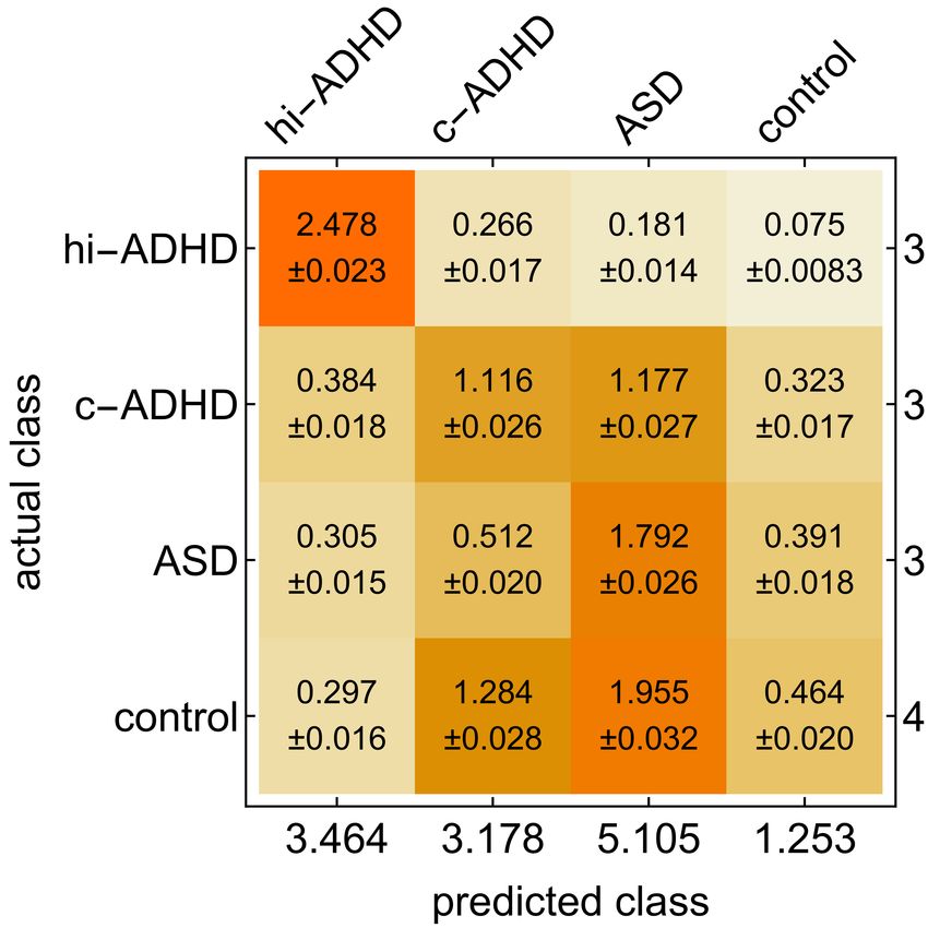
2

                                                      I.   INTRODUCTION

   Mathematical analysis of physiological signals, human movement variability among them, for decades attracted considerable
attention of the scientific community, resulting in a large body of available methods (see, references [1, 2], which are still
not exhaustive). This paper takes advantage of this aggregated wealth, gathers multiple quantifiable characteristics of human
actigraphy records, and takes them as input for supervised machine-learning algorithms in order to help in diagnosing and
differentiating Attention Deficit Hyperactivity Disorder (ADHD) in children.
   Actigraphs are wristwatch-like devices that use accelerometers to register locomotor activity. The analysis of the data they
provide is frequently considered a cost-effective method of first choice, used both in clinical research and practice. Since motor
activity levels and circadian rhythms are related to a range of psychiatric disorders [3], their monitoring can be utilized in
diagnosis, prediction of treatment response or for sleep assessment. Beside sleep and major mood disorders some neurological
diseases such as Parkinson’s disease [4–6], vascular dementia [7], Alzheimer’s disease [3, 8], schizophrenia [9] or chronic
pain [10] have been shown to be related to abnormal activity symptoms.
   In terms of nosological classification, ADHD is a separate disease entity, whose diagnostic criteria are included in DSM-5 [11]
and ICD-10 [12]. The behavioral symptoms included as criteria for ADHD are attention disorders, psychomotor hyperactivity,
and impulsiveness. Attention disorders are predominantly connected to a lowered ability to concentrate and to keep attention on
a given task, which include, lowered selectivity as well as excessive susceptibility to distractors. Hyperactivity manifests itself
by heightened motor activity, usually chaotic, and undertaken without precise aim or purpose. Impulsiveness on the other hand
is connected to a person behaving to stimuli occurring at a given time, however, without reflecting on its adequacy or potential
effects. Depending on the intensity of the motor and attention focus symptoms, DSM-5 differentiates between three subtypes of
ADHD:

    • ADHD-predominantly inattentive type - presents with being easily distracted, forgetful, daydreaming, disorganization,
      poor concentration, and difficulty completing tasks;

    • ADHD-predominantly hyperactive-impulsive type, henceforth denote for short ‘hi-ADHD’ – presents with excessive fid-
      getiness and restlessness, hyperactivity, difficulty waiting and remaining seated, and immature behavior, where destructive
      behaviors may also be present;

    • ADHD combined type, henceforth denoted ‘c-ADHD’ – is a combination of the first two subtypes.

In general, the results of neuropsychological tests used in ADHD research rely on various simultaneous cognitive functions,
which as a rule, do not indicate the specific neuronal circuits which malfunction in ADHD persons [13]. However, such opportu-
nities have been presented by some research paradigms developed by combining experimental psychology and neurobiological
approaches together with advanced mathematical methods of bioelectrical brain activity measurements, and other experimental
and neuroimaging techniques. These paradigms include among others, auditory and visual oddball tasks [14–16], as well as
actigraphy studies. A review of previous research on actigraphy records revealed [17–20] that ADHD children were shown to
exhibit increased motor activity during sleep and increased nocturnal activity in studies using actigraphy. At the same time,
it was reported [21] that the results concerning the nature of the sleep and activity problems in ADHD children are unclear
due to methodological limitations of the studies. A large part of what is currently known about attention-deficit/hyperactivity
disordered children’s functioning in sleep is based on ADHD Combined Type samples, but there is little research focused on
experimentally differentiating the other ADHD subtypes [19, 22], where behavioral data analysis can be verified with relatively
sensitive measurements, and interpreted with the use of sophisticated statistical models.
   A common approach to analyze such a record is to inspect activity profiles or histograms, extract circadian frequency and
phase shifts, sleep duration and wake after sleep onset or to reduce the time series to a summary statistic such as mean activity
level, ratio of nocturnal and diurnal activity, or intra- and interdaily variability, etc. [3, 8, 23, 24]. While such measures allow
employing classic statistical methods, more relevant information may be exposed when other advanced tools of quantification,
like fractal analysis, are applied [4–6, 25–27]. Specifically, the power law exponent describing temporal autocorrelations of
activity correlates with the symptoms of some disorders or conditions. Similar scaling laws have been found in activity period
distributions in humans suffering from major depressive disorders [28, 29] and individuals subject to sleep deprivation [25, 26,
30]. Disruption of these laws in the context of rest and activity fluctuations in light and dark phases of the circadian cycle was
further studied by [31].
   In this paper we refrain from delving into hypothetical sources and theoretical repercussions of these results. The focus is on
which quantities and to what extent can avail diagnosis of hyperactivity disorders in children. In Methods Section we lay out
the relevant details on the measurements and the subjects, as well as on some simple stages of preprocessing the collected data.
Next, we list and discuss all the quantities applied for characterizing the individual time series. We explain meaning and details
of computing these quantities only briefly, whenever we can refer to existing studies. Finally, Results Section reports on the
results of classifying the subjects into different groups. These results are followed with a discussion and conclusions in the last
section.
3

                                                         II.     METHODS

                                                        A.      Study design

   Participants were registered and diagnosed in respective clinics before commencement of the study. Participants and their
parents were informed about the procedure and goals of the study, and provided their written consent for the actigraphic and
supplementary psychological examination (including WISC-R). Participant selection was based on medical and psychological
records. Next, a 7 day actigraphic recording was performed. The key quantities (classification features) were designed before
obtaining the data; the cross-validation paradigm was designed after the data had been collected based on their size. The study
was approved by the Bioethics Commission at Jagiellonian University. In order to minimize any potential discomfort, anxiety
and other psychological costs related to participation in the study, the caregivers could phone and consult a member of the team
(clinical psychologist) at every stage of the experiment, they were provided detailed instructions, and encouraged to ask any
questions and express any concerns.

                                                         B.     Participants

   The ADHD participants were identified in registry of a local (Skawina near Kraków, Poland) specialized educational psy-
chology clinic. The ASD participants were identified at a local (Kraków, Poland) autism and developmental disorders clinic
and had been diagnosed by a medical doctor (psychiatrist) and a clinical psychologist. In this study, including the ASD group
serves mainly as a way of testing robustness of the classifiers’ specificity in a scenario with multiple disorders to diagnose. The
control group was randomly selected from among boys attending regular primary schools located in the same area from where
the subjects with developmental disorders lived. The participants had not undergone any pharmacotherapy up to six months
prior to the study.
   The exclusion criteria before actigraphy recording were: ambiguous ADHD symptoms, suspected co-occurring developmental
disorders (ADHD and ASD groups), below normal intelligence assessment (all groups). The control group was comprised of
children showing no psychological disorders, nor any other serious somatic diseases; they also came from families that did not
reveal pathological traits or characteristics.
   The ADHD diagnosis was obtained in accordance with the current standards of assessment [11, 12]. It involved an expert
assessing the intensity levels of symptoms in the areas of hyperactivity, impulsiveness and attention deficit, according to the
diagnostic criteria of DSM-5 [11]. The assessment was based on clinical observations, as well as, information obtained from
the parents and the child during a diagnostic interview. Intellectual functioning of all subjects was determined with the WISC-R
scale. The study involves and relates to the children with the ADHD combined type and the hyperactive-impulsive type only.
Due to developmental aspects, it would be inappropriate to the inattentive ADHD type, as children in this group aged 8-10, have
a tendency to alter the intensity of the dominant symptoms of ADHD, as reported in [32–36].

                                                       C.      Actigraphy data

   All subjects were given a motor activity recording device – Micro Motionlogger SleepWatch (Ambulatory Monitoring, Inc.,
Ardsley, NY), to be worn continuously (without being taken off at night or during bathing) on the wrist of the non-dominant
hand. Recording time took no longer than 7 days. The subjects did not perform any additional tasks or tests, and participated
in their normal daily activities during this period. The parents were instructed to inform the research team of any infections
of the participants and any medication taken during the recording. The actigraph activity monitors were personally put on and
taken off each subject by a member of the research team. Three hyperactive-impulsive participants reported displeasure due
to wearing the devices during sleep. The data were collected continuously in 1-minute epochs with the Zero Crossing Mode
(ZCM), see Fig. 1(A), and Proportional Integrating Measure (PIM) mode. In short, the ZCM mode measures frequency of
movements and the PIM mode a quantity proportional to energy expenditure. ZCM counts the number of times per epoch that
the transducer signal crosses a positive threshold close to zero; e.g., raising a hand in a single smooth movement would give 2
ZCM counts during the acceleration phase and 0 during deceleration, totaling 2 counts for the movement. In this mode high
frequency artefacts may potentially be misinterpreted as considerable motion. PIM integrates the total area under the absolute
value of the signal curve in a given epoch, giving an integer number in the range [0,65535] representing the sum of momentum
changes. For the movement described above it would add both the acceleration and deceleration.
   Raw actigraph records were cut into days and nights by finding peaks in Pearson correlation of ZCM with a step function and
subsequent human verification. Individual days were excluded from the records on visual inspection due to non-compliance of
some subjects to wear the device. At the group level, all days of clean data were taken into account (9% of daily records were
removed due to non-compliance of some subjects to wear the device). The total numbers of analyzed daily records were 41,
33, 32, and 42 for control, combined subtype, hyperactive-impulsive subtype, and ASD, respectively. Below, whenever we refer
C   Actigraphy data                                                                                                                           4

           A                                                                                                         C

           B                                                                                                         D

FIG. 1. (A) Raw Zero Crossing Mode (ZCM) measurements and (B) standardized increments ∆ZCM for an hi-ADHD subject, with black
and red indicating diurnal and nocturnal activity. Right panels (C, D) show histograms of activity for the most distinctive subjects in all four
groups; horizontal axes indicates probability density, vertical axes are the same as in panels (A, B).

to days and nights, we mean 14-hour diurnal and 4-hour nocturnal (before wake-up) actigraphy record, which is to normalize
lengths of the samples and avoid possible artifacts due to differing sleep lengths. The details of further processing are described
below.

                                                            D.   Selected features

 There are in total 47 features of time series that we used for classification. Here we briefly introduce them, from least to the
most complex, and refer to Appendix A for more details.

    • Sleep (1-3): waking hour, hour of falling asleep and the duration of sleep.

    • Statistics of activity (4-11), Fig. 2: we computed 2 × 2 × 2 = 8 parameters: average and standard deviation of activity at
      night and during day in ZCM and PIM modes. That these quantities can be reasonable candidate parameters for prediction
      can be inferred from inspecting differences between activity histograms of extreme individuals visible in Fig. 2.

    • Statistics of increments of activity (12-15): kurtosis of ZCM/PIM diurnal/nocturnal activity increments. Taking increments
      (i.e., differences between consecutive time points) effectively removes slow changes in a time series, which is often
      desirable in further analysis. The peakedness of distributions of increments, which can be quantified as kurtosis, can be
      observed in lower right panel in Fig. 1.

    • Return maps (16-19): the ZCM and PIM positions of the fixed points and the square deviation of the ZCM and PIM curves
      from the diagonal on the return map plot (in which we plot a series at time t against the same series at t + 1). In short, the
      fixed points are the states to which the system is ultimately drawn (like activity and rest in ZCM actigraphic series), and
      the deviations mentioned above are a proxy for the speed of returning to these states. Return maps have been used, e.g., in
      movement analysis in ants [37].

    • Hurst exponent (20-23): subject averages of ZCM/PIM exponents over days/nights. They were computed with detrended
      fluctuation analysis (DFA) [38, 39], frequently used in analysis of physiological data [25, 40–43]. The Hurst exponent is
      especially known in analysis of fractal time series. It is a flagship example a measure for long-term memory of a process.

    • Durations of activity and rest (24-31): the average duration of activity/rest, and α and γ parameters for both ZCM and
      PIM modes. Activity and rest periods were defined as actigraphy measurements lying above or below a predefined thresh-
      old (see Fig. 1 upper panel). It has been shown that in humans and other species the durations a have complementary
      cumulative distributions C(a) of universal shapes [29, 44], a power-law C(a) = a−γ for rest and a stretched exponential
D Selected features 5
FIG. 2. Density histograms of activity of the individual subjects chosen from each group. (A) control, (B) autism spectrum disorder, (C)
ADHD combined type, (D) ADHD-predominantly hyperactive-impulsive type. Each colored pixel denotes how often a given subject engaged
in an activity with a given Zero Crossing Mode (ZCM) and Proportional Integrating Measure (PIM) intensity. Compare with histograms for
ZCM in Fig. 1.
C(a) = exp −αaβ for activity periods. The parameters of these distributions can differ between conditions such as
major depressive disorder, chronic sleep deprivation or schizophrenia [9, 26, 28, 30].
• Average shape of activity (32-35): skewness of the shapes for ZCM and PIM, and the scaling exponents µ. By the
shape we mean the curve ZCM(t) (or PIM(t)) taking an excursion above a predefined, low threshold. In humans and
ants [37, 45] such excursions follow some universal, approximately parabolic shapes [46, 47], see Fig. 4. The scaling
exponent µ describes the scaling between durations T of the excursions and their sizes S. The disorders under study could
hypothetically manifest themselves as deviations from such universality of these quantities.
• Non-linear forecasting features (36-39): the skewed difference statistic [48] and the non-linear prediction error [49, 50]D Selected features 6
60 000
Control 60 000
hi-ADHD
40 000 40 000
PIM(t+1)
PIM(t+1)
20 000 20 000
0 0
0 20 000 40 000 60 000 0 20 000 40 000 60 000
PIM(t) PIM(t)
FIG. 3. Return maps in PIM mode for most distinctive individuals in control and hi-ADHD groups. x-axis is activity at time t and y-axis is
the activity in the next time step. Red circles show averages over bins of equal number of data points. Red arrows indicate the crossing point
between the map and the diagonal.
1.0
0.8
106 hi-ADHD
0.6 μ+1
⟨PIM⟩/T μ
c-ADHD
⟨S⟩
0.4
ASD
5
10
control
0.2
5 10 20 50
0.0 T
0.0 0.2 0.4 0.6 0.8 1.0
t/T
FIG. 4. Average shape of Proportional Integrating Measure (PIM) activity (feature 8) of the most distinctive individuals from each group.
Inset: universal scaling between durations T of excursions and their average sizes S, with the scaling exponent µ.
for ZCM and PIM. These measures are known in non-linear forecasting. Their intuitive meaning is as follows: the first
measures the size of asymmetry between rises and falls of a numerical sequence; the second measures how well a model
predicts activity at time t + T , given the activity at time t.
• Lempel-Ziv complexity [51] (40-47): for diurnal and nocturnal ZCM and PIM activity and their increments. This infor-
mation theoretical quantity measures irregularity or randomness of a sequence, and is reduced by its repetitiveness. We
used the simplest version of the algorithm for binary sequences, which involved binarization of the actigraphic records
(for diurnal ZCM and PIM, substituting activity below mean with zeros and above with ones; for nocturnal records, all
non-zero activity was turned into ones; the series of increments were binarized into positive and non-negative).B Feature correlations 7
E. Optimizing feature subset
In this study, since both the size of the data set and the feature set are small, we performed a brute-force search for subset
of features optimizing classification performance: first, we computed performance of all (1,081) feature pairs and ranked them
according to their median accuracy (in a 4-class task); we chose twelve highest scoring but least correlated features; ultimately,
an exhaustive search was performed over all (3,797) combinations of up to eight out of the twelve best features.
F. Classifier
Since we resorted to exhaustive search, we utilized naïve Bayes classifier due to its speed. After finding the final near optimal
feature sets, we checked whether other classifiers (all implemented by default in Mathematica 11.3: nearest neighbor, logistic
regression, support vector machines and random forest) improve on naïve Bayes’s performance. Ultimately, the best results that
we report on, see Table I, include logistic regression, naïve Bayes, nearest neighbor.
G. Cross-validation
The sensitivity and specificity results are averages (and standard deviations) based on 100 cross-validation runs. In the 4-class
(control, ASD, c-ADHD, hi-ADHD) and 3-class task (control, c-ADHD, hi-ADHD) task the scores were calculated as weighted
averages over non-control classes. In the 4-class task and 3-class task, for a given feature set each run consisted of randomly
assigning four subjects from each group to the training set, and the three-four remaining ones to the test set. In the binary
classification task (control versus both ADHD subtypes), in each run four control subjects, two c-ADHD and two hi-ADHD
were sampled to both the training and test set, in order to retain balance between sample sizes. We classified subjects only on
the level of a person (based on all available days) and not on the level of days per person, because some of the features need a
larger statistic to be feasible for estimation.
III. RESULTS
In the previous section we presented in total 47 features that hypothetically can give insight into the nature of hyperactivity as
measured by means of actigraphy. Below we show how these features were used to train a classifier that, given a new subject,
can label him or her as belonging to one of the four groups: control, ASD, c-ADHD, and hi-ADHD.
A. Participants
This study involved n=29 male participants, aged 9.89 ± 0.92 years, in four groups (7 with c-ADHD, 7 with hi-ADHD,
7 with autism spectrum disorder, ASD, and 8 in the control). There were 48 potentially eligible participants; 18 participants
were excluded due to suspected co-occurring developmental disorders, and one participant was excluded due to below normal
intelligence assessment. The actigraphy was recorder between in Nov-Dec 2015 (ASD), Feb and June 2016 (ADHD groups),
Feb-March 2016 and one person in July 2016 (control); the time of year has marginal interaction with the classification results.
The subjects in ADHD groups had been under psychological counselling for 3.4 ± 2.4 years at the time of actigraphy recording.
There were no clinical interventions between or during enrollment and data collection; no medication use was reported.
B. Feature correlations
Understandably, with only 29 subjects this big number of features can lead to undesirable effects, like overfitting the clas-
sifier. However, since a lot of the features are by design strongly interrelated, we can reduce their number and obtain a better
understanding of what they indicate. We used a weighted-average agglomerative clustering algorithm searching for six feature
clusters, which we list and discuss below (feature numbers correspond to the order of presentation in Section “Methods: Se-
lected features”; for visual representation of feature correlation matrix see Fig. 5(left) below, and Fig. 5(right) for the clustered
correlation matrix):
A (4, 8) mean daytime activity ZCM and PIM, (12) daytime ZCM kurtosis of increments, (17-18) return map crossing
PIM and return map deviation ZCM, (24, 26, 28, 30) mean active and resting durations of ZCM and PIM, (36) skewed
difference in ZCM;B Feature correlations 8
B (2) hour of falling asleep, (13) daytime PIM kurtosis of increments, (21) daytime DFA exponent PIM, (25,29) active
durations exponent ZCM and PIM, (31) resting durations exponent PIM, (34-35) µ exponent ZCM and PIM;
C (14-15) nocturnal kurtosis of ZCM and PIM increments;
D (20) daytime DFA exponent ZCM, (32) shape skewness ZCM, (37-39) skewed difference in PIM and prediction error in
ZCM and PIM;
E (1, 3) waking hour and sleep time, (8) std. dev. of daytime activity PIM, (16) return map crossing ZCM, (19) return map
deviation PIM, (33) shape skewness PIM, (40-47) all Lempel-Ziv complexities;
F (6, 10) mean activity at night ZCM and PIM, (7, 11) std. dev. of activity at night ZCM and PIM, (22-23) night DFA
exponent ZCM and PIM, (27) resting durations exponent ZCM.
1 3 5 7 9 11 13 15 17 19 21 23 25 27 29 31 33 35 37 39 41 43 45 47 12 8 26 30 17 13 35 5 25 31 15 20 38 33 1 16 40 42 44 46 22 6 10 27
2 4 6 8 10 12 14 16 18 20 22 24 26 28 30 32 34 36 38 40 42 44 46 4 24 28 18 36 34 21 2 29 14 32 37 39 9 3 19 41 43 45 47 23 7 11
1 12
2 4
3 8
4 24
5
7
6
26
30
28 A
8
correlation
18
9 17 1.0
10 36
11 13
12 34
13 35
14 21
15
16
5
2
B 0.5
17 25
18 29
19 31
20
21
22
15
14
32
C
23 20
25
24
26
38
37 D 0
27
39
28
33
29
9
30 1
31 3
32 16
19 -0.5
33
35
34 40
42
41 E
36
37 43
38 44
39 45
40 46 -1.0
41 47
42 22
43 23
6
45
44
46 10
7 F
47 11
sleep increments Hurst exponents shape complexity 27
acitivity return maps durations forecasting
FIG. 5. Left: correlation matrix of all the 47 features. Right: correlation matrix rearranged into six clusters of highly correlated features. The
feature numbers, as described in text, are provided for reference. The triangles on the sides point to the eight selected features; red triangles
indicate the four performing best.
The groups A and B are very strongly anti-correlated, which for classifying purposes means they both bear similar information
content. Similarly, group C is anti-correlated to group F. All the Lempel-Ziv complexities in group E are very strongly correlated
with each other but at the same time they are anti-correlated with groups D and F. There is a noteworthy likeness, expected in
theory, between DFA exponents, exponents of distributions of rest and activity durations, and the scaling exponents µ (cluster
B). Notably, the highly (anti-)correlated clusters A and B do not contain features informative for classification purposes. The
best features, cf. Table I, especially in cluster D, are rather weakly correlated among themselves but also to all other features.
C. Best features
The eight best performing feature subsets together with their classification algorithms, selected as described in Section “Meth-
ods: Selected features”, are listed in Table I. Most importantly, the best feature, shape skewness in ZCM mode on its own leads
to a significantly non-random result with accuracy: 41.38 ± 1.1% (against 25% chance baseline). Combinations of remaining
features incrementally enhance performance as shown in Table I.
The best nearest neighbors 4-feature classifier reached 46.5 ± 1.1% accuracy (against 25% chance baseline), 61.8 ± 1.4%
sensitivity and 79.30 ± 0.43% specificity in a 4-class task (control, ASD, hi-ADHD, c-ADHD). The same classifier obtained
62.6 ± 1.9% sensitivity and 70.1 ± 9.8% specificity in a 3-class task (control, hi-ADHD, c-ADHD) and 69.4 ± 1.6% accuracy
(against 50% chance baseline) 78.0 ± 2.2% sensitivity and 60.8 ± 2.6% specificity in a binary task; please note that this classifier
had been optimized for four-class problem. Tests on the final feature sets indicate that logistic regression systematically obtainsC Best features 9
Classifier NB LR LR NN LR LR LR LR
Sensitivity [%] 43.6 ± 1.3 50.7 ± 1.3 51.4 ± 1.4 61.8 ± 1.4 53.0 ± 1.2 49.6 ± 1.4 53.4 ± 1.2 53.3 ± 1.5
Specificity [%] 79.67 ± 0.70 80.03 ± 0.59 82.43 ± 0.64 79.30 ± 0.43 82.73 ± 0.50 80.63 ± 0.62 81.30 ± 0.59 82.07 ± 0.50
No Group
32 D + + + + + + + +
1 E + + + + + +
14 C + + + + +
39 D + + + + +
37 D + + + +
38 D + + +
27 F + + +
45 E + +
TABLE I. The eight best scoring classifiers; highest scores are in bold, and the frame indicates the selected best classifier. The values
of sensitivity and specificity are averages ± standard deviation of the mean. The ’+’ signs in columns indicate 1-8 features included in a
classifier. Classifier names: LR – logistic regression, NN – nearest neighbors, NB – naïve Bayes. Feature names: 32 – Zero Crossing Mode
(ZCM) shape skewness, 1 – waking hour, 14 – nocturnal kurtosis of ZCM increments, 39 – Proportional Integrating Measure (PIM) prediction
error, 37 – PIM skewed difference, 38 – ZCM prediction error, 27 – ZCM exponent of resting times γ, 45 – Lempel-Ziv complexity of PIM
increments. Groups refer to correlation clusters, Sec. III B.
similar scores. Due to large deviations (the provided uncertainties are standard deviations of the mean of 100 cross-validation
tests), however, it is not possible to provide the one and only significantly better classifier or feature set. It is worth noting that
out of the features belonging to the correlated groups A and B none were selected.
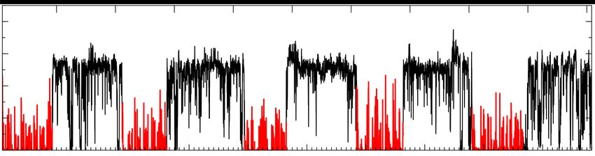
In Fig. 6 we supplement the results with the whole confusion matrix for the 4-feature nearest neighbors classifier using on
both the 4-class and binary problem obtained after 1,000 cross-validation runs. The predictions for hi-ADHD are very good and
are promising for ASD. Strikingly, the controls are often misclassified as either ASD or c-ADHD condition, and the c-ADHD
group is in turn often misclassified as ASD. This serves as a cautionary example that some features might not be specific to one
disorder only. In the binary case, the classifier is highly sensitive to the ADHD condition.
A B
FIG. 6. (A) Confusion matrix in a 4-class task of the best 4-feature classifier; (B) confusion matrix in a binary task (control vs ADHD) with
the same classifier. Numbers are means and standard deviations of the mean in a 1,000 cross-validation setup. The diagonal entries are the
correctly classified cases, the off-diagonal are misclassified cases. Numbers on the axes are row and column sums.C Best features 10
IV. DISCUSSION AND CONCLUSIONS
The results presented in this paper indicate that advanced analysis of actigraphy measurements can enhance diagnostics of
hyperactivity disorders in children. In a realistic setting patients may differ in type and intensity of disorder symptoms (like
ADHD subtypes), as well as they can actually suffer from another disorder (here, the ASD group was used as a convenient
way of further confusing the classifiers). For these reasons we believe that a classifier successfully tested on multiple classes is
reliable and it might be general enough to distinguish in a controlled setting also other disorders.
Merely one quantity is enough to produce results better than chance: the skewness of the averaged shape of activity of a
person. The results show that also other selected quantities are informative, e.g., non-linear forecasting measures (prediction
error and skewed difference), the peakedness of the histogram of differenced nocturnal activity, or simply a person’s waking
hour. These might offer clues as to the nature of symptoms in hyperactivity disorders. They can also already improve diagnosis
of these disorders, especially with the use of wearable telemetric devices.
Further experimental studies should explore how to observe differences in symptom intensity in children with ADHD com-
bined subtype and hyperactivity-impulsiveness subtype as they relate to the changes in parameters and topography in both
hemispheres of the event-related potential connected to the process of categorizing new and known stimuli. This proposed con-
text of differentiation between ADHD subtypes would not only be more precise, but would also provide new interdisciplinary
perspectives for therapeutic interventions for this disorder.
Actigraphy results, supported by appropriate mathematical interpretations, could be useful for detecting subclinical deficits
in the subtypes. Analysis of the obtained results showed that such a method can effectively differentiate between children with
specific ADHD subtypes and those without ADHD, and that it allows for the detection of subtle disorders of motor activity,
as well as, indirectly, cognitive processing abilities. Therefore, it seems legitimate to consider actigraphy in addition to the
analysis of event-related potentials when diagnosing ADHD, in order to make an unambiguous diagnosis, and to avoid running
into serious difficulties when preparing to provide appropriate and effective therapeutic intervention strategies.
ACKNOWLEDGMENTS
JKO thanks Valeria Pattacini from the Office of International Relations of Universidad de San Martín, UNSAM, (Argentina)
for facilitating his visit and the UNSAM’s hospitality. We would like to thank Anna Bereś at the Institute of Applied Psychology,
Jagiellonian University, for discussions on study design at the initial stages of the project, and Maria Marczyk from “Effatha”
Centre for Autistic People, for the acquisition of data from ASD-diagnosed children. Work conducted under the auspice of the
Jagiellonian University-UNSAM Cooperation Agreement. JKO was supported by the Grant DEC-2015/17/D/ST2/03492 of the
National Science Centre (Poland). DRC was supported in part by CONICET (Argentina) and Escuela de Ciencia y Tecnología,
UNSAM.
Appendix A: Methods supplement
Sleep
Three straightforward quantities connected with sleep were taken into account: waking hour, hour of falling asleep and the
duration of sleep. Obviously, they are dependent, but it is not a priori clear which of them can be most informative. The
differences between the groups indicated in Tab. II show that they can be of moderate use at the prediction stage.
Waking Falling asleep Sleep duration
ASD c-ADHD hi-ADHD ASD c-ADHD hi-ADHD ASD c-ADHD hi-ADHD
control 0.63 0.20 0.078 0.23 0.98 0.060 0.11 0.14 0.39
ASD 0.19 0.33 0.19 0.0061 0.026 0.054
c-ADHD 0.018 0.039 0.53
TABLE II. P-values (< 0.05 in bold) of two-sided Student’s t-tests for differences between the experimental groups in waking time, time of
falling asleep and the duration of sleep.11
Statistics of activity
The starting point of the data analysis was a visual inspection of activity histograms of the extreme individuals visible in
Fig. 2. The activity included five days trimmed to 4 hours of sleep (before wake-up) followed by 14 hours of daytime (the
trimming is performed to avoid possible effects due to differing sleep lengths, which are treated separately). It is easy to
notice that ADHD subject (and similarly the ASD subject) has a relatively higher volume of activity around ZCM = 260 and
P IM = 20000 − 45000, while the main control subject’s activity lies in the region ZCM < 200 and P IM < 10000, and
the c-ADHD subject is intermediate between the two. The high probability in the yellow pixel around 0 is a result of the low
nocturnal activity.
The above observations allow to assume that mean and standard deviation of activity (that is roughly the location and spread
of activity in Fig. 2) are reasonable candidate parameters for prediction. Thus we computed 2 × 2 × 2 = 8 parameters: average
and standard deviation for night and day in ZCM and PIM mode separately. For each subject the average and standard deviation
were calculated from concatenation of all the valid 4-hour (or 14-hour) periods.
Additionally, when examining the set of all the subjects with each day and night treated separately, the mean presented strong
anticorrelations with variance in ZCM day, and strong correlation in ZCM and PIM nights, see Table III. This behavior can
be understood in terms of the universal shape of the activity histograms (e.g., at night whenever non-zero activity occurs, the
variance naturally rises).
control ASD c-ADHD hi-ADHD
ZCM day < -0.61 -0.70 -0.61 -0.74
ZCM night > 0.95 0.65 0.76 0.92
PIM night > 0.94 0.75 0.85 0.93
TABLE III. Correlations between mean and variance of activity; p-value < 0.05, Spearman one-sided test for correlation coefficient being
lower/greater than the given value. For PIM day the correlations are insignificant or weak.
Statistics of increments of activity
Removing slow changes in a time series can be helpful in further analysis. It can be achieved simply by differencing the raw
time series, resulting in a series of activity increments, as shown in Fig. 1.It appears that not only the histograms of raw activity
differ between the groups, as discussed earlier, but also the histograms of increments. As shown in Fig. 1 (lower right panel),
the extreme subjects from different groups exhibited varying peakedness of such histograms. This can be simply measured by
kurtosis of the increment distributions. Consequently, we included another four features for classification purposes: kurtosis of
PIM/ZCM diurnal/nocturnal differenced activity.
Return map
Based already on Fig. 2 it is visible that one can define two states, especially for hyperactive subjects: resting (around zero
ZCM and PIM values) and active (spread around ZCM = 260 and P IM = 30000). These points can be found by means of so
called return (or Poincaré) maps that have been used, e.g., in movement analysis in ants [37].
Given a series at time t, we plot it against the same series one step forward at t + 1, see Fig. 3. If the obtained line were a
diagonal, it would mean that starting from any activity at time t the subject would remain with the same value of activity in the
next time step. If the obtained line crosses the diagonal, as it does in Fig. 3 around P IM = 30000 for ADHD, it is a fixed point
of the activity. In this case, it means that the activity in some range below and above ultimately makes its way towards that point,
and the speed of that travel depends on the crossing angle. Mark that there is another fixed point at null activity.
From these considerations another four features were computed: the ZCM and PIM positions of the crossing (of an interpo-
lated curve with the diagonal), and the square deviation of the curves from the diagonal (as a more robust proxy for the estimate
of the crossing angle).
Hurst exponent
We further consider properties known from analysis of fractal time series. A flagship example is the Hurst exponent, measuring
long-term memory of a process. It can be estimated by several interrelated methods like Fano factor and Allan variance (see,12
e.g., [26, 52, 53]), wavelet analysis and other ones. We decided to turn to the detrended fluctuation analysis (DFA) [38, 39],
frequently used in analysis of physiological data [25, 40–43].
The scaling exponents were obtained separately for each 14-hour day and 4-hour night. The basic DFA variant was computed
with only linear trends removed. For a given subject, the features used were: average of ZCM/PIM exponents over days/nights.
Durations of activity and rest
Another set of properties of interest – very much related to the concept above – concerns inter-event periods [53, 54]. In
particular, if an event is defined as the moment of activity crossing a given threshold, the inter-event periods become the durations
of high activity and rest (above and below the threshold, respectively). It has been shown that in humans and other species the
durations a have complementary cumulative distributions C(a) of universal shapes [29, 44], a power-law C(a) = a−γ for
β
rest and a stretched exponential C(a) = exp −αa for activity periods; the precise form of the distribution can be further
improved [55]. Moreover, the parameters of these distributions can differ between conditions such as major depressive disorder,
chronic sleep deprivation or schizophrenia [9, 26, 28, 30].
There are eight features that were extracted from inter-event period lengths: the average duration of activity/rest, and α and γ
parameters for both ZCM and PIM modes. The first quantity, the average period duration, has been used [29, 44] as a rescaling
factor that allowed distributions to conform to a universal shape; thus in itself it might be indicative of individual characteristics
of the time series. Here we computed it for each day separately and averaged over all days for a given subject. The parameters
α and γ were fitted using log-log or log-linear data for power-law and stretched exponential, respectively, in order to account for
the tails in the distributions. For a better stability of the stretched exponential fit the other parameter was set to a constant, rough
estimate β = 0.5. For a given subject, the fit was performed on joint data from all available days.
Average shape of activity
Apart from all the statistics described above, it is reasonable to assume that simply the shape the time course of activity can
differ between individuals or conditions. By the shape we mean the curve ZCM (t) (or P IM (t)) taking an excursion above a
predefined threshold. It has been shown for humans and ants [37, 45] that such excursions follow some universal, approximately
parabolic shapes [46, 47], see Fig. 4. To obtain this result one has to first determine the scaling between durations T of the
excursions and their sizes S. Upon visual inspection it became apparent that despite similar form the shapes can be skewed
towards beginning or the end of the excursion.
We therefore included as additional four features: skewness of the shapes for ZCM and PIM, as well as the scaling exponents
µ. The quantities were computed with ZCM = 100 and P IM = 10000 activity thresholds, and jointly out of all available days
for a given subject.
Prediction error
Furthermore, we compute two measures known in non-linear forecasting: one is the skewed difference statistic [48]
3
h(xt+T − xt ) i
Q(T ) = 2 , (A1)
h(xt+T − xt ) i
and the other is the non-linear prediction error [49, 50]
2
h(ft,T − xt+T ) i
E 2 (T ) = 2 , (A2)
h(xt − x̄) i
where xt is a given time series, x̄ is its time average, T is the number of time steps ahead we try to predict, and ft,T is the
function we construct to predict the behavior at time t + T given some knowledge at time t.
The intuitive meaning for the first measure is the size of asymmetry between rises and falls. In the simplest case, linearly
increasing activity produces Q(T ) ∼ T , while linearly decreasing activity Q(T ) ∼ −T . If an activity is roughly constant, but it
tends to rise up or fall down after some given time T , this would likewise be reflected in Q. Since one of our hypotheses is that
the shape of activity might differ between healthy and disordered people, as already indicated in Sec. A, it is a valid measure to
investigate.
The prediction error is technically much more involved, although simple conceptually: given some activity at time t we want
to predict it at time t + T , we construct a model with the prediction ft,T and check it against the real future activity. If the model
is simply the average activity x̄t , the error will be equal to E 2 = 1; if the prediction is perfect, E 2 = 0.13
ZCM
100 PIM
10 000
50 5000
0
0
-5000
Q
Q
control -10 000 control
-50
ASD ASD
-15 000
-100 c-ADHD c-ADHD
-20 000
hi-ADHD hi-ADHD
-150 -25 000
0 100 200 300 400 500 0 100 200 300 400 500
lag [minutes] lag [minutes]
ZCM PIM
4000
10
0 2000
-10
0
-20
Q
Q -2000
-30
control control
ASD -4000 ASD
-40
c-ADHD -6000 c-ADHD
-50
hi-ADHD hi-ADHD
-60 -8000
0 100 200 300 400 500 0 100 200 300 400 500
lag [minutes] lag [minutes]
FIG. 7. Skewed difference (A1) for ZCM and PIM modes on (upper panels) single individuals and (lower panels) group level. From each day
only 12-hour long stretch of daily activity was taken.
Note that our goal here is actually not to optimize the predictions or to test for non-linearity, but to simply examine if for
a given model the prediction error will be informative of the activity disorder. To that purpose we use a somewhat arbitrary,
but a very straightforward following model. We divide the recordings into training and test set; we take an hour-long piece
Xt = {x0t }tt0 =t−60 from the test set and ask for a prediction 20 minutes in the future {xt0 }t+20
t0 =t+1 ; in the training set, we find an
ensemble of k = 5 hour-long pieces which look most similar to Xt , which we call nearest neighbors, {Yi,t }ki=1 . The prediction
Pk
is given simply by the average f (t, T ) = 1/k i=1 yi,t+T .
Both the skewed difference and prediction error are functions of T . For the purpose of classification, instead of functions
we preferred single numbers, so we used average scores (over the range T = 1 − 500 for Q(T ) and T = 1 − 20 for E 2 (T ),
respectively, as presented in Fig. 7-8). For a given subject in ZCM/PIM mode, the features were calculated for each day
separately and subsequently were averaged.
[1] M. Akay, Nonlinear Biomedical Signal Processing Vol. II: Dynamic Analysis and Modeling (Wiley-IEEE Press, 2000).
[2] N. Stergiou, ed., Nonlinear analysis for human movement variability (Taylor & Francis Group, 2016).
[3] M. H. Teicher, Harvard review of psychiatry 3, 18 (1995).
[4] W. Pan, K. Ohashi, Y. Yamamoto, and S. Kwak, Movement disorders 22, 1308 (2007).
[5] W. Pan, S. Kwak, F. Li, C. Wu, Y. Chen, Y. Yamamoto, and D. Cai, Physiology & behavior 119, 156 (2013).
[6] Y. Sun, C. Wu, J. Wang, and W. Pan, Int. J. Integrative Medicine 1, 1 (2013).
[7] W.-D. Pan, S. Yoshida, Q. Liu, C.-L. Wu, J. Wang, J. Zhu, and D.-F. Cai, Translational Neurodegeneration 2, 9 (2013).
[8] E. J. van Someren, E. E. Hagebeuk, C. Lijzenga, P. Scheltens, S. E. de Rooij, C. Jonker, A.-M. Pot, M. Mirmiran, and D. F. Swaab,
Biological Psychiatry 40, 259 (1996).14
ZCM PIM
5 5
control control
4 4
ASD ASD
prediction error
prediction error
c-ADHD c-ADHD
3 3
hi-ADHD hi-ADHD
2 2
1 1
0 0
0 5 10 15 20 0 5 10 15 20
time of prediction [minutes] time of prediction [minutes]
FIG. 8. Prediction error (A2) for ZCM and PIM modes on most distinctive individuals. From each day only 10-hour long stretch of daily
activity was taken. The prediction error values above three in the hi-ADHD subject in ZCM are not representative of the whole group.
[9] W. Sano, T. Nakamura, K. Yoshiuchi, T. Kitajima, A. Tsuchiya, Y. Esaki, Y. Yamamoto, and N. Iwata, PloS ONE 7, e43539 (2012).
[10] A. C. Long, T. M. Palermo, and A. M. Manees, Journal of Pediatric Psychology 33, 660 (2008).
[11] A. P. Association. and A. P. Association., Diagnostic and statistical manual of mental disorders : DSM-5, 5th ed. (American Psychiatric
Association Arlington, VA, 2013) pp. xliv, 947 p. ;.
[12] W. H. Organization., The ICD-10 classification of mental and behavioural disorders : diagnostic criteria for research (World Health
Organization Geneva, 1993) pp. xiii, 248 p. ;.
[13] J. A. Sergeant, H. Geurts, and J. Oosterlaan, Behavioural brain research 130, 3 (2002).
[14] J. R. Folstein and C. Van Petten, Psychophysiology 45, 152 (2008).
[15] S. J. Johnstone, R. J. Barry, and A. R. Clarke, International Journal of Psychophysiology 66, 37 (2007).
[16] M. Senderecka, A. Grabowska, K. Gerc, J. Szewczyk, and R. Chmylak, International Journal of Psychophysiology 85, 106 (2012).
[17] M. G. Melegari, E. Vittori, L. Mallia, A. Devoto, F. Lucidi, R. Ferri, and O. Bruni, Journal of attention disorders , 1087054716672336
(2016).
[18] F. De Crescenzo, S. Licchelli, M. Ciabattini, D. Menghini, M. Armando, P. Alfieri, L. Mazzone, G. Pontrelli, S. Livadiotti, F. Foti, et al.,
Sleep medicine reviews 26, 9 (2016).
[19] S. Wiebe, J. Carrier, S. Frenette, and R. Gruber, Journal of sleep research 22, 41 (2013).
[20] V. Moreau, N. Rouleau, and C. M. Morin, Behavioral sleep medicine 12, 69 (2014).
[21] A. Poirier and P. Corkum, Journal of attention disorders , 1087054715575065 (2015).
[22] S. P. Becker, L. J. Pfiffner, M. A. Stein, G. L. Burns, and K. McBurnett, Sleep medicine 21, 151 (2016).
[23] H. Oginska, J. Mojsa-Kaja, M. Fafrowicz, and T. Marek, Journal of sleep research 23, 341 (2014).
[24] L. Matuzaki, R. Santos-Silva, E. C. Marqueze, C. R. de Castro Moreno, S. Tufik, and L. Bittencourt, Sleep Science 7, 152 (2014).
[25] P. M. Holloway, M. Angelova, S. Lombardo, A. S. C. Gibson, D. Lee, and J. Ellis, Journal of The Royal Society Interface 11, 20131112
(2014).
[26] E. Gudowska-Nowak, J. K. Ochab, K. Oleś, E. Beldzik, D. R. Chialvo, A. Domagalik, M. Fafrowicz,
˛ T. Marek, M. A. Nowak, H. Ogińska,
J. Szwed, and J. Tyburczyk, Journal of Statistical Mechanics: Theory and Experiment 2016, 054034 (2016).
[27] P. Wohlfahrt, J. W. Kantelhardt, M. Zinkhan, A. Y. Schumann, T. Penzel, I. Fietze, F. Pillmann, and A. Stang, EPL (Europhysics Letters)
103, 68002 (2013).
[28] T. Nakamura, K. Kiyono, K. Yoshiuchi, R. Nakahara, Z. Struzik, and Y. Yamamoto, Phys. Rev. Lett. 99, 138103 (2007).
[29] T. Nakamura, T. Takumi, A. Takano, N. Aoyagi, K. Yoshiuchi, Z. Struzik, and Y. Yamamoto, PloS ONE 3, e2050 (2008).
[30] J. K. Ochab, J. Tyburczyk, E. Beldzik, D. R. Chialvo, A. Domagalik, M. Fafrowicz, E. Gudowska-Nowak, T. Marek, M. A. Nowak,
H. Oginska, and J. Szwed, PLOS ONE 9, 1 (2014).
[31] A. Proekt, J. Banavar, A. Maritan, and D. Pfaff, Proc. Natl. Acad. Sci. USA 109, 10564 (2012).
[32] H. I. Kaplan and B. J. Sadock, Synopsis of psychiatry: Behavioral sciences clinical psychiatry (Williams & Wilkins Co, 1988).
[33] W. M. Klykylo and J. Kay, Clinical child psychiatry (John Wiley & Sons, 2006).
[34] M. E. Lewis, Child and adolescent psychiatry: A comprehensive textbook (Lippincott Williams & Wilkins Publishers, 2002).
[35] D. Semple and R. Smyth, Oxford handbook of psychiatry (OUP Oxford, 2013).
[36] B. Lask, S. Taylor, and K. P. Nunn, Practical child psychiatry (BMJ Publishing Group, 2003).
[37] R. Gallotti and D. R. Chialvo, Journal of The Royal Society Interface 15 (2018), 10.1098/rsif.2018.0223.
[38] C.-K. Peng, S. V. Buldyrev, S. Havlin, M. Simons, H. E. Stanley, and A. L. Goldberger, Physical review e 49, 1685 (1994).
[39] P. Talkner and R. O. Weber, Physical Review E 62, 150 (2000).
[40] E. Rodriguez, J. C. Echeverria, and J. Alvarez-Ramirez, Physica A: Statistical Mechanics and its Applications 384, 429 (2007).15
[41] D. Makowiec, A. Rynkiewicz, R. Gałaska, J. Wdowczyk-Szulc, and M. Żarczyńska-Buchowiecka, EPL (Europhysics Letters) 94, 68005
(2011).
[42] J. Gierałtowski, D. Hoyer, F. Tetschke, S. Nowack, U. Schneider, and J. Żebrowski, Autonomic Neuroscience: Basic and Clinical 178,
29 (2013).
[43] G. Şahin, M. Erentürk, and A. Hacinliyan, Chaos, Solitons & Fractals 41, 198 (2009).
[44] C. Anteneodo and D. Chialvo, Chaos: An Interdisciplinary Journal of Nonlinear Science 19, 033123 (2009).
[45] D. Chialvo, A. M. G. Torrado, E. Gudowska-Nowak, J. K. Ochab, P. Montoya, M. A. Nowak, and E. Tagliazucchi, Papers in physics 7,
070017 (2015).
[46] A. Baldassarri, F. Colaiori, and C. Castellano, Physical review letters 90, 060601 (2003).
[47] F. Colaiori, A. Baldassarri, and C. Castellano, Physical Review E 69, 041105 (2004).
[48] J. Theiler, S. Eubank, A. Longtin, B. Galdrikian, and J. D. Farmer, Physica D: Nonlinear Phenomena 58, 77 (1992).
[49] J. D. Farmer and J. J. Sidorowichl, in Evolution, learning and cognition (World Scientific, 1988) pp. 277–330.
[50] A. Longtin, BME 11, 11 (1997).
[51] A. Lempel and J. Ziv, IEEE Transactions on information theory 22, 75 (1976).
[52] S. Thurner, S. B. Lowen, M. C. Feurstein, C. Heneghan, H. G. Feichtinger, and M. C. Teich, Fractals 5, 565 (1997).
[53] C. Anteneodo, R. D. Malmgren, and D. Chialvo, The European Physical Journal B 75, 389 (2010).
[54] D. R. Bickel, Physica A: Statistical Mechanics and its Applications 265, 634 (1999).
[55] J. J. Chapman, J. A. Roberts, V. T. Nguyen, and M. Breakspear, Scientific reports 7, 43174 (2017).You can also read