Compact Deep Aggregation for Set Retrieval
←
→
Page content transcription
If your browser does not render page correctly, please read the page content below
Compact Deep Aggregation for Set Retrieval
                                         Yujie Zhong · Relja Arandjelović · Andrew Zisserman
arXiv:2003.11794v1 [cs.CV] 26 Mar 2020

                                         Abstract The objective of this work is to learn a compact              such as a group of friends or a family. Then we would like the
                                         embedding of a set of descriptors that is suitable for efficient       retrieved images that contain all of the set to be ranked first,
                                         retrieval and ranking, whilst maintaining discriminability of          followed by images containing subsets, e.g. if there are three
                                         the individual descriptors. We focus on a specific example of          friends in the query, then first would be images containing
                                         this general problem – that of retrieving images containing            all three friends, then images containing two of the three,
                                         multiple faces from a large scale dataset of images. Here the          followed by images containing only one of them. Consider
                                         set consists of the face descriptors in each image, and given          another example where a fashion savvy customer is research-
                                         a query for multiple identities, the goal is then to retrieve, in      ing a dress and a handbag. A useful retrieval system would
                                         order, images which contain all the identities, all but one, etc.      first retrieve images in which models or celebrities wear both
                                              To this end, we make the following contributions: first,          items, so that the customer can see if they match. Following
                                         we propose a CNN architecture – SetNet – to achieve the ob-            these, it would also be beneficial to show images containing
                                         jective: it learns face descriptors and their aggregation over a       any one of the query items so that the customer can discover
                                         set to produce a compact fixed length descriptor designed for          other fashionable combinations relevant to their interest. For
                                         set retrieval, and the score of an image is a count of the num-        these systems to be of practical use, we would also like this
                                         ber of identities that match the query; second, we show that           retrieval to happen in real time.
                                         this compact descriptor has minimal loss of discriminability                These are examples of a set retrieval problem: the database
                                         up to two faces per image, and degrades slowly after that – far        consists of many sets of elements (e.g. the set is an image
                                         exceeding a number of baselines; third, we explore the speed           containing multiple faces, or of a person with multiple fash-
                                         vs. retrieval quality trade-off for set retrieval using this com-      ion items), and we wish to order the sets according to a query
                                         pact descriptor; and, finally, we collect and annotate a large         (e.g. multiple identities, or multiple fashion items) such that
                                         dataset of images containing various number of celebrities,            those sets satisfying the query completely are ranked first
                                         which we use for evaluation and is publicly released.                  (i.e. those images that contain all the identities of the query,
                                         Keywords Image retrieval · Set retrieval · Face recognition ·          or all the query fashion items), followed by sets that satisfy
                                         Descriptor aggregation · Representation learning · Deep                all but one of the query elements, etc. An example of this
                                         learning                                                               ranking for the face retrieval problem is shown in Fig. 1 for
                                                                                                                two queries.
                                                                                                                    In this work, we focus on the problem of retrieving a set
                                         1 Introduction                                                         of identities, but the same approach can be used for other
                                                                                                                set retrieval problems such as the aforementioned fashion
                                         Suppose we wish to retrieve all images in a very large collec-         retrieval. We can operationalize this by scoring each face in
                                         tion of personal photos that contain a particular set of people,       each photo of the collection as to whether they are one of the
                                                                                                                identities in the query. Each face is represented by a fixed
                                         Y. Zhong and A. Zisserman
                                         Visual Geometry Group, Department of Engineering Science, University
                                                                                                                length vector, and identities are scored by logistic regression
                                         of Oxford, UK                                                          classifiers. But, consider the situation where the dataset is
                                         E-mail: {yujie,az}@robots.ox.ac.uk                                     very large, containing millions or billions of images each
                                         R. Arandjelović                                                       containing multiple faces. In this situation two aspects are
                                         DeepMind                                                               crucial for real time retrieval: first, that all operations take
                                         E-mail: relja@google.com                                               place in memory (not reading from disk), and second that an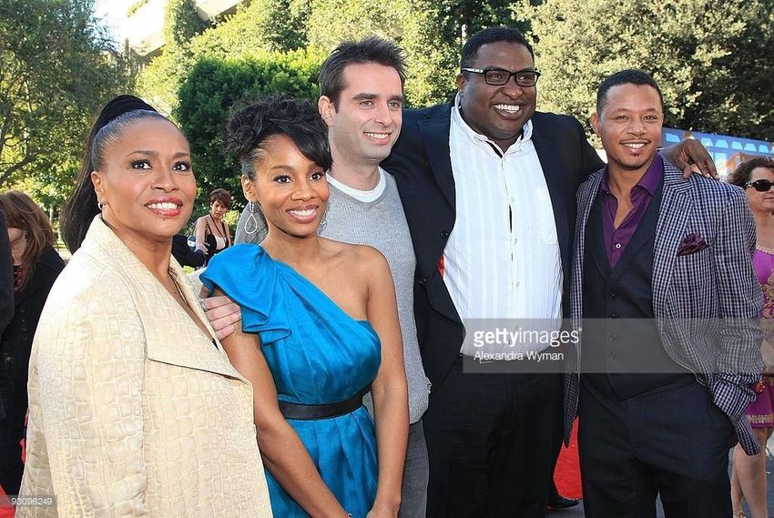
2 Y. Zhong, R. Arandjelović and A. Zisserman
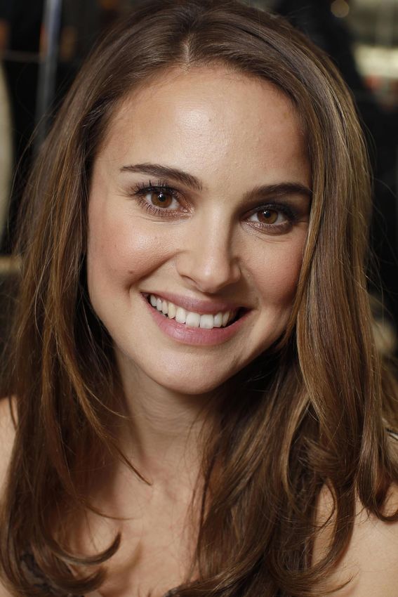
Query: Top 3 Query: Top 3
Barbara Hershey
Martin Freeman
Natalie Portman
Mark Gatiss
Vincent Cassel
Fig. 1: Images ranked using set retrieval for two example queries. The query faces are given on the left of each example
column, together with their names (only for reference). Left: a query for two identities; right: a query for three identities. The
first ranked image in each case contains all the faces in the query. Lower ranked images partially satisfy the query, and contain
progressively fewer faces of the query. The results are obtained using the compact set retrieval descriptor generated by the
SetNet architecture, by searching over 200k images of the Celebrity Together dataset introduced in this paper.
efficient algorithm is used when searching for images that is small, typically 128 (to keep the memory footprint low),
satisfy the query. The problem is that storing a fixed length and N is in the thousands.
vector for each face in memory is prohibitively expensive We make the following contributions: first, we introduce
at this scale, but this cost can be significantly reduced if a a trainable CNN architecture for the set-retrieval task that
fixed length vector is only stored for each set of faces in an is able to learn to aggregate face vectors into a fixed length
image (since there are far fewer images than faces). As well descriptor in order to minimize interference, and also is able
as reducing the memory cost this also reduces the run time to rank the face sets according to how many identities are
cost of the search since fewer vectors need to be scored. in common with the query using this descriptor. To do this,
So, the question we investigate in this paper is the fol- we propose a paradigm shift where we draw motivation from
lowing: can we aggregate the set of vectors representing the image retrieval based on local descriptors. In image retrieval,
multiple faces in an image into a single vector with little it is common practice to aggregate all local descriptors of
loss of set-retrieval performance? If so, then the cost of both an image into a fixed-size image-level vector representa-
memory and retrieval can be significantly reduced as only tion, such as bag-of-words (Sivic and Zisserman, 2003) and
one vector per image (rather than one per face) have to be VLAD (Jégou et al., 2010); this brings both memory and
stored and scored. speed improvements over storing all local descriptors indi-
Although we have motivated this question by face re- vidually. We generalize this concept to set retrieval, where
trieval it is quite general: there is a set of elements (which instead of aggregating local interest point descriptors, set ele-
are permutation-invariant), each element is represented by ment descriptors are pooled into a single fixed-size set-level
a vector of dimension De , and we wish to represent this set representation. For the particular case of face set retrieval,
by a single vector of dimension D, where D = De in practice, this corresponds to aggregating face descriptors into a set
without losing information essential for the task. Of course, representation. The novel aggregation procedure is described
if the total number of elements in all sets, N, is such that in Sec. 3 where the aggregator can be trained in an end-to-end
N ≤ D then this certainly can be achieved provided that the manner with different feature extractor CNNs.
set of vectors are orthogonal. However, we will consider the Our second contribution is to introduce a dataset anno-
situation commonly found in practice where N
D, e.g. D tated with multiple faces per images. In Sec. 4 we describe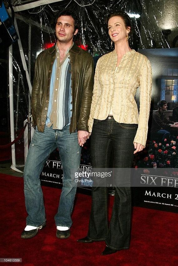
Compact Deep Aggregation for Set Retrieval                                                                                          3

a pipeline for automatically generating a labelled dataset of            VLAD has recently been adapted into a differentiable
pairs (or more) of celebrities per image. This Celebrity To-         CNN layer, NetVLAD (Arandjelović et al., 2016), making
gether dataset contains around 200k images with more than            it end-to-end trainable. We incorporate a modified form of
half a million faces in total. It is publicly released.              the NetVLAD layer in our SetNet architecture. An alterna-
    The performance of the set-level descriptors is evaluated        tive, but related, very recent approach is the memory vector
in Sec. 5. We first ‘stress test’ the descriptors by progressively   formulation proposed by Iscen et al. (2017), but we have not
increasing the number of faces in each set, and monitoring           employed it here as it has not been made differentiable yet.
their retrieval performance. We also evaluate retrieval on the
Celebrity Together dataset, where images contain a variable
number of faces, with many not corresponding to the queries,         2.2 Image retrieval
and explore efficient algorithms that can achieve immediate
(real-time) retrieval on very large scale datasets. Finally, we      Another strand of research we build on is category level
investigate what the trained network learns by analyzing why         retrieval, where in our case the category is a face. This is an-
the face descriptors learnt by the network are well suited for       other classical area of interest with many related works (Chat-
aggregation.                                                         field et al., 2011; Perronnin et al., 2010b; Torresani et al.,
    Note, although we have grounded the set retrieval prob-          2010; Wang et al., 2010; Zhou et al., 2010). Since the advent
lem as faces, the treatment is quite general: it only assumes        of deep CNNs (Krizhevsky et al., 2012), the standard solution
that dataset elements are represented by vectors and the scor-       has been to use features from the last hidden layer of a CNN
ing function is a scalar product. We return to this point in the     trained on ImageNet (Donahue et al., 2013; Razavian et al.,
conclusion.                                                          2014; Sermanet et al., 2013) as the image representation.
                                                                     This has enabled a very successful approach for retrieving im-
                                                                     ages containing the query category by training linear SVMs
2 Related work                                                       on-the-fly and ranking images based on their classification
                                                                     scores(Chatfield et al., 2014, 2015). For the case of faces, the
To the best of our knowledge, this paper is the first to consider    feature vector is produced from the face region using a CNN
the set retrieval problem. However, the general area of image        trained to classify or embed faces (Parkhi et al., 2015; Schroff
retrieval has an extensive literature that we build on here.         et al., 2015; Taigman et al., 2014). Li et al. (2011) tackle face
                                                                     retrieval by using binary codes that jointly encode identity
                                                                     discriminability and a number of facial attributes. Li et al.
2.1 Aggregating descriptors                                          (2015) extend image-based face retrieval to video scenarios,
                                                                     and learn low-dimensional binary vectors encoding the face
One of the central problems that has been studied in large           tracks and hierarchical video representations.
scale image instance retrieval is how to condense the informa-           Apart from single-object retrieval, there are also works
tion stored in multiple local descriptors such as SIFT (Lowe,        on compound query retrieval, such as (Zhong et al., 2016)
2004), into a single compact vector to represent the image.          who focus on finding a specific face in a place. While this
This problem has been driven by the need to keep the mem-            can be seen as set retrieval where each set has exactly two
ory footprint low for very large image datasets. An early            elements, one face and one place, it is not applicable to our
approach is to cluster descriptors into visual words and rep-        problem as their elements come from different sources (two
resent the image as a histogram of word occurrences – bag-           different networks) and are never combined together in a
of-visual-words (Sivic and Zisserman, 2003). Performance             set-level representation.
can be improved by aggregating local descriptors within each
cluster, in representations such as Fisher Vectors (Jégou et al.,
2011; Perronnin et al., 2010a) and VLAD (Jégou et al., 2010).       2.3 Approaches for sets
In particular, VLAD – ‘Vector of Locally Aggregated De-
scriptors’ by Jégou et al. (2010) and its improvements (Arand-      Also relevant are works that explicitly deal with sets of vec-
jelović and Zisserman, 2013; Delhumeau et al., 2013; Jégou         tors. Kondor and Jebara (2003) developed a kernel between
and Zisserman, 2014) was used to obtain very compact de-             vector sets by characterising each set as a Gaussian in some
scriptions via dimensionality reduction by PCA, consider-            Hilbert space. However, their set representation cannot cur-
ably reducing the memory requirements compared to earlier            rently be combined with CNNs and trained in an end-to-end
bag-of-words based methods (Chum et al., 2007; Nister and            fashion. Feng et al. (2017) learn a compact set representation
Stewenius, 2006; Philbin et al., 2007; Sivic and Zisserman,          for matching of image sets by jointly optimizing a neural net-
2003). VLAD has superior ability in maintaining the infor-           work and hashing functions in an end-to-end fashion. Pooling
mation about individual local descriptors while performing           architectures are commonly used to deal with sets, e.g. for
aggressive dimensionality reduction.                                 combining information from a set of views for 3D shape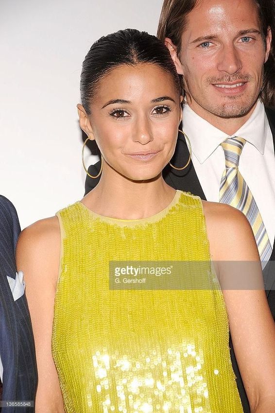
4                                                                                         Y. Zhong, R. Arandjelović and A. Zisserman

recognition (Shi et al., 2015; Su et al., 2015). Zaheer et al.     and this naturally orders the images by the number of faces
(2017) investigate permutation-invariant objective functions       it contains that satisfy the query.
for operating on sets, although their method boils down to         Network Deployment. To deploy the set level descriptor for
average pooling of input vectors, which we compare to as a         retrieval in a large scale dataset, there are two stages:
baseline. Some works adopt attention mechanism (Ilse et al.,       Offline: SetNet is used to compute face descriptors for each
2018; Lee et al., 2018; Vinyals et al., 2016; Yang et al., 2018)   face in an image, and aggregate them to generate a set-vector
or relational network (Santoro et al., 2017) into set opera-       representing the image. This procedure is carried out for
tions to model the interactions between elements in the input      every image in the dataset, so that each image is represented
set. Hamid Rezatofighi et al. (2017) consider the problem          by a single vector.
of predicting sets, i.e. having a network which outputs sets,      At run-time, to search for an identity, a face descriptor is
rather than our case where a set of elements is an input to be     computed for the query face using SetNet, and a logistic
processed and described with a single vector. Siddiquie et al.     regression classifier used to score each image based on the
(2011) formulate a face retrieval task where the query is a set    scalar product between its set-vector and the query face de-
of attributes. Yang et al. (2017) and Liu et al. (2017) learn      scriptor. Searching with a set of identities amounts to sum-
to aggregate set of faces of the same identity for recognition,    ming up the image scores of each query identity.
with different weightings based on image quality using an
attention mechanism. For the same task, Wang et al. (2017)
represent face image sets as covariance matrices. Note, our        3.1 SetNet architecture
objective differs from these: we are not aggregating sets of
faces of the same identity, but instead aggregating sets of        In this section we introduce our CNN architecture, designed
faces of different identities.                                     to aggregate multiple element (face) descriptors into a single
                                                                   fixed-size set representation. The SetNet architecture (Fig. 2)
                                                                   conceptually has two parts: (i) each face is passed through a
3 SetNet – a CNN for set retrieval                                 feature extractor network separately, producing one descrip-
                                                                   tor per face; (ii) the multiple face descriptors are aggregated
As described in the previous section, using a single fixed-        into a single compact vector using a modified NetVLAD
size vector to represent a set of vectors is a highly appealing    layer, followed by a trained dimensionality reduction. At
approach due to its superior speed and memory footprint over       training time, we add a third part which emulates the run-
storing a descriptor-per-element. In this section, we propose      time use of logistic regression classifiers. All three parts of
a CNN architecture, SetNet, for the end-task of set retrieval.     the architecture are described in more detail next.
There are two objectives:                                          Feature extraction. The first part is a CNN for feature ex-
1. It should learn the element descriptors together with the       traction which produces individual element descriptors (x1
aggregation in order to minimise the loss in face classification   to xF ), where F is the number of faces in an image. We ex-
performance between using individual descriptors for each          periment with two different base architectures – modified
face, and an aggregated descriptor for the set of faces. This      ResNet-50 (He et al., 2016) and modified SENet-50 (Hu
is achieved by training the network for this task, using an        et al., 2018), both chopped after the global average pooling
architecture combining ResNet for the individual descriptors       layer. The ResNet-50 and SENet-50 are modified to produce
together with NetVLAD for the aggregation.                         De dimensional vectors (where De is 128 or 256) in order to
2. It should be able to rank the images using the aggregated       keep the dimensionality of our feature vectors relatively low,
descriptor in order of the number of faces in each image that      and we have not observed a significant drop in face recogni-
correspond to the identities in the query. This is achieved        tion performance from the original 2048-D descriptors. The
by scoring each face using a logistic regression classifier.       modification is implemented by adding a fully-connected
Since the score of each classifier lies between 0 and 1, the       (FC) layer of size 2048× De after the global average pooling
score for the image can simply be computed as the sum of           layer of the original network, in order to obtain a lower De -
the individual scores, and this summed score determines the        dimensional face descriptor. This additional fully-connected
ranking function.                                                  layer essentially acts as a dimensionality reduction layer. This
     As an example of the scoring function, if the search is       modification introduces around 260k additional weights to
for two identities and an image contains faces of both of          the network for De = 128, and 520k weights for De = 256,
them (and maybe other faces as well), then the ideal score         which is negligible compared to the total number of param-
for each relevant face would be one, and the sum of scores         eters of the base networks (25M for ResNet-50, 28M for
for the image would be two. If an image only contains one of       SENet-50).
the identities, then the sum of the scores would be one. The       Feature aggregation. Face features are aggregated into a
images with higher summed scores are then ranked higher            single vector V using a NetVLAD layer (illustrated in Fig. 3,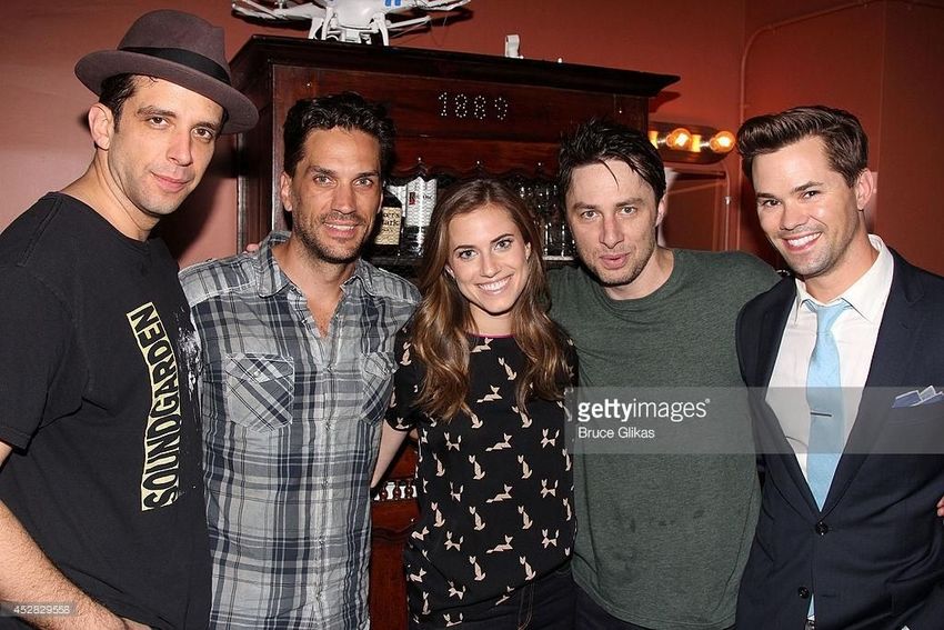
Compact Deep Aggregation for Set Retrieval                                                                                                     5

                               SetNet                                                             SetNet Deployment
                                                                                                        score ∈ (0,1)

                                                                                                              logistic regression classifier
             set representation:           set   (D)                                                   Sigmoid

                                                                                              Scale (w) and Shift (b)
                                                            aggregator
                              BN & L2N

                                                                                                    scalar product
                           FC (De x K) x D                                          set                                        q

                                                                                                                                                   V4
                            Vset         (De x K)
                                                                                    SetNet                                     SetNet

                                   L2N

                    NetVLAD Layer (K clusters)
                                                                                  dataset image                             query face

                                                                                                  Baseline Network

                                                                                                      set

                       1             2                  3
                                                                                                            L2N

                                                                feature
                                                               extractor                              Avg Pooling
                     L2N           L2N                 L2N                                                                                              CN

                                                                                                                                    feature
                                                                                          L2N               L2N          L2N
                                                                                                                                   extractor
                    CNN            CNN              CNN

                                                                                          CNN               CNN         CNN

Fig. 2: SetNet architecture and training. Left: SetNet – features are extracted from each face in an image using a modified
ResNet-50 or SENet-50. They are aggregated using a modified NetVLAD layer into a single De × K dimensional vector
which is then reduced to D dimension (where D is 128 or 256) via a fully connected dimensionality reduction layer, and
L2-normalized to obtain the final image-level compact representation. Right (top): at test time, a query descriptor, vq , is
obtained for each query face using SetNet (the face is considered as a single-element set), and the dataset image is scored by a
logistic regression classifier on the scalar product between the query descriptor vq and image set descriptor vset . The final
score of an image is then obtained by summing the scores of all the query identities. Right (bottom): the baseline network
has the same feature extractor as SetNet, but the feature aggregator uses an average-pooling layer, rather than NetVLAD.

and described below in Sec. 3.2). The NetVLAD layer is                     to NetVLAD. The NetVLAD-pooled features are reduced
slightly modified by adding an additional L2-normalization                 to be D-dimensional by means of a fully-connected layer
step – the total contribution of each face descriptor to the               followed by batch-normalization (Ioffe and Szegedy, 2015),
aggregated sum (i.e. its weighted residuals) is L2-normalized              and L2-normalized to produce the final set representation
in order for each face descriptor to contribute equally to                 vset .
the final vector; this procedure is an adaptation of residual
                                                                           Training block. At training time, an additional logistic re-
normalization (Delhumeau et al., 2013) of the vanilla VLAD
                                                                           gression loss layer is added to mimic the run-time scenario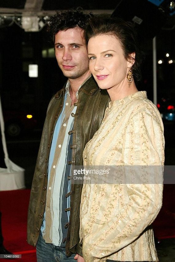
6                                                                                                            Y. Zhong, R. Arandjelović and A. Zisserman

                           soft-assignment
                                                                                     in the image, and zero for the other P − F faces. The loss
x1, …, xF                                                                    V
             conv(a, b)
                                         soft-max            aggregation
                                                                                     measures the deviation from this ideal score, and the network
            1x1xDxK
                                                                                     learns to achieve this by maintaining the discriminability for
                                                                                     individual face descriptors after aggregation.
              residual                                           L2
            computation                      X               normalization               In detail, incorporating the loss is achieved by adding
                                                                                     an additional layer at training time which contains a logistic
                                                                                     regression loss for each of the P training identities, and is
Fig. 3: NetVLAD layer. Illustration of the NetVLAD                                   trained together with the rest of the network.
layer (Arandjelović et al., 2016), corresponding to equation
                                                                                     Multi-label logistic regression loss. For each training image
(1), and slightly modified to perform L2-normalization before
                                                                                     (set of faces), the loss L is computed as:
aggregation; see Sec. 3.2 for details.

                                                                                              P
where a logistic regression classifier is used to score each                         L = − ∑ y f log(σ (w(vTf vset ) + b))+
image based on the scalar product between its set-vector and                                 f =1                                                   (2)
the query face descriptor. Note, SetNet is used to generate                             (1 − y f ) log(1 − σ (w(vTf vset ) + b))
both the set-vector and the face descriptor. Sec. 3.3 describes
the appropriate loss and training procedure in more detail.                          where σ (s) = 1/(1 + exp(−s)) is a logistic function, P is the
                                                                                     number of face descriptors (the size of the mini-batches at
                                                                                     training), and w and b are the scaling factor and shifting bias
3.2 NetVLAD trainable pooling                                                        respectively of the logistic regression classifier, and y f is a
                                                                                     binary indicator whether face f is in the image or not. Note
NetVLAD has been shown to outperform sum and max pool-                               that multiple y f ’s are equal to 1 if there are multiple faces
ing for the same vector dimensionality, which makes it per-                          which correspond to the identities in the image.
fectly suited for our task. Here we provide a brief overview
of NetVLAD, for full details please refer to (Arandjelović
et al., 2016).
                                                                                     3.4 Implementation details
    For F D-dimensional input descriptors {xi } and a chosen
number of clusters K, NetVLAD pooling produces a single                              This section gives full details of the training procedure, in-
D × K vector V (for convenience written as a D × K matrix)                           cluding how the network is used at run-time to rank the
according to the following equation:                                                 dataset images given query examples.
                       T
            F
                    eak xi +bk                                                       Training data. The network is trained using faces from the
V ( j, k) = ∑                         (xi ( j) − ck ( j)),    j ∈ 1, . . . , D (1)
                       aTk0 xi +bk0                                                  training partition of the VGGFace2 dataset (Cao et al., 2018).
            i=1   ∑k 0 e
                                                                                     This consists of 8631 identities, with on average 360 face
where {ak }, {bk } and {ck } are trainable parameters for k ∈                        samples for each identity.
[1, 2, . . . , K]. The first term corresponds to the soft-assignment                 Balancing positives and negatives. For each training image
weight of the input vector xi for cluster k, while the second                        (face set) there are many more negatives (the P − F identities
term computes the residual between the vector and the cluster                        outside of the image set) than positives (identities in the
centre. Finally, the vector is L2-normalized.                                        set), i.e. most y f ’s in eq. (2) are equal to 0 with only a few
                                                                                     1’s. To restore balance, the contributions of the positives
                                                                                     and negatives to the loss function is down-weighted by their
3.3 Loss function and training procedure
                                                                                     respective counts.
In order to achieve the two objectives outlined at the begin-                        Initialization and pre-training. A good (and necessary) ini-
ning of Sec. 3, a Multi-label logistic regression loss is used.                      tialization for the network is obtained as follows. The face
Suppose a particular training image contains F faces, and                            feature extraction block is pretrained for single face classi-
the mini-batch consists of faces for P identities. Then in a                         fication on the VGGFace2 Dataset (Cao et al., 2018) using
forward pass at training time, the descriptors for the F faces                       softmax loss. The NetVLAD layer, with K = 8 clusters, is
are aggregated into a single feature vector, vset , using the                        initialized using k-means as in (Arandjelović et al., 2016).
SetNet architecture, and a face descriptor, v f , is computed                        The fully-connected layer, used to reduce the NetVLAD di-
using SetNet for each of the faces of the P identities. The                          mensionality to D, is initialized by PCA, i.e. by arranging the
training image is then scored for each face f by applying a                          first D principal components into the weight matrix. Finally,
logistic regressor classifier to the scalar product vTset v f , and                  the entire SetNet is trained for face aggregation using the
the score should ideally be one for each of the F identities                         Multi-label logistic regression loss (Sec. 3.3).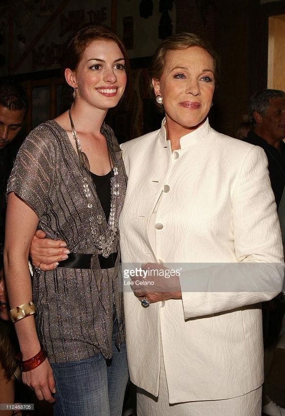
Compact Deep Aggregation for Set Retrieval                                                                                        7

Training details. Training requires face set descriptors com-       much more complex than when building a single-face-per-
puted for each image, and query faces (which may or may             image dataset, such as (Parkhi et al., 2015). The straightfor-
not occur in the image). The network is trained on synthetic        ward strategy of (Parkhi et al., 2015), which involves simply
face sets which are built by randomly sampling identities (e.g.     searching for celebrities on an online image search engine, is
two identities per image). For each identity in a synthetic set,    inappropriate: consider an example of searching for Natalie
two faces are randomly sampled (from the average of 360             Portman on Google Image Search – all top ranked images
for each identity): one contributes to the set descriptor (by       contain only her and no other person. Here we explain how to
combining it with samples of the other identities), the other       overcome this barrier to collect images with multiple celebri-
is used as a query face, and its scalar product is computed         ties in them.
with all the set descriptors in the same mini-batch. In our         Query selection. In order to acquire celebrity name pairs, we
experiments, each mini-batch contains 84 faces. Stochastic          first perform a search by using ‘seed-celebrity and’,
gradient descent is used to train the network (implemented          and then scan the meta information for other celebrity names
in MatConvNet (Vedaldi and Lenc, 2015), with weight decay           to produce a list of (seed-celebrity, celebrity-friend) pairs.
0.001, momentum 0.9, and an initial learning rate of 0.001          However, one important procedure which is not included
for pre-training and 0.0001 for fine-tuning; the learning rates     in the main paper is that some celebrity may have a strong
are divided by 10 in later epochs.                                  connection to one or more particular celebrities, which could
    Faces are detected from images using MTCNN (Zhang               prevent us from obtaining a diverse list of celebrity friends.
et al., 2016). Training faces are resized such that the smallest    For instance, almost all the top 100 images returned by ‘Be-
dimension is 256 and random 224 × 224 crops are used as             yoncé and’ are with her husband Jay Z. Therefore, to pre-
inputs to the network. To further augment the training faces,       vent such celebrity friends dominating the top returned re-
random horizontal flipping and up to 10 degree rotation is          sults, a secondary search is conducted by explicitly removing
performed. At test time, faces are resized so that the smallest     pairs found by the first-round search, i.e. the query term
dimension is 224 and the central crop is taken.                     now is ‘seed-celebrity and -friend1 -friend2
Dataset retrieval. Suppose we wish to retrieve images con-          ...’, where friend1, friend2 .. are those found in the
taining multiple identities (or a subset of these). First, a face   first search. We do not perform more searches after the sec-
descriptor is produced by SetNet for each query face. The           ond round, as we find that the number of new pairs obtained
face descriptors are then used to score a dataset image for         in the third-round search is minimal.
each query identity, followed by summing the individual             Image download and filtering. Once the name pairs are
logistic regression scores to produce the final image score.        obtained, we download the images and meta information
A ranked list is obtained by sorting the dataset images in          from the image search engine, followed by name scanning
non-increasing score order. In the case where multiple face         again to remove false images. Face detection is performed
examples are available for a query identity, SetNet is used to      afterwards to further refine the dataset by removing images
extract face descriptors and aggregate them to form a richer        with fewer than two faces.
descriptor for that query identity.
                                                                    De-duplication. Removal of near duplicate images is per-
                                                                    formed similarly to (Parkhi et al., 2015), adapted to our case
4 ‘Celebrity Together’ dataset                                      where images contain multiple faces. Namely, we extract a
                                                                    VLAD descriptor for each image (computed using densely
A new dataset, Celebrity Together, is collected and annotated.      extracted SIFT descriptors (Lowe, 2004)) and cluster all im-
It contains images that portray multiple celebrities simultane-     ages for each celebrity. This procedure results in per-celebrity
ously (Fig. 4 shows a sample), making it ideal for testing set      clusters of near duplicate images. Dataset-wide clustering
retrieval methods. Unlike the other face datasets, which ex-        is obtained as the union of all per-celebrity clusters, where
clusively contain individual face crops, Celebrity Together is      overlapping clusters (i.e. ones which share an image, which
made of full images with multiple labelled faces. It contains       can happen because images contain multiple celebrities) are
194k images and 546k faces in total, averaging 2.8 faces per        merged. Finally, de-duplication is performed by only keeping
image. The image collection and annotation procedures are           a single image from each cluster. Furthermore, images in
explained next.                                                     common with the VGG Face Dataset (Parkhi et al., 2015) are
                                                                    removed as well.
                                                                    Image annotation. Each face in each image is assigned to
4.1 Image collection and annotation procedure                       one of 2623 classes: 2622 celebrity names used to collect the
                                                                    dataset, or a special “unknown person” label if the person is
The dataset is created with the aim of containing multiple peo-     not on the predefined celebrity list; the “unknown” people
ple per image, which makes the image collection procedure           are used as distractors.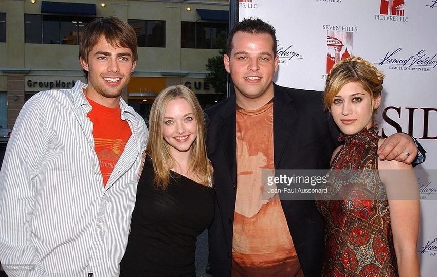
8                                                                                           Y. Zhong, R. Arandjelović and A. Zisserman

     (a)                              (b)                      (c)                                 (d)

    (e)                             (f)                              (g)                              (h)

    (i)                               (j)                           (k)                                  (l)

Fig. 4: Example images of the Celebrity Together Dataset. Note that only those celebrities who appear in the VGG Face
Dataset are listed, as the rest are labelled as ‘unknown’. (a) Amy Poehler, Anne Hathaway, Kristen Wiig, Maya Rudolph. (b)
Bingbing Fan, Blake Lively. (c) Kat Dennings, Natalie Portman, Tom Hiddleston. (d) Kathrine Narducci, Naturi Naughton,
Omari Hardwick, Sinqua Walls. (e) Helena Christensen, Karolina Kurkova, Miranda Kerr. (f) Adam Levine, Blake Shelton,
CeeLo Green. (g) Aamir Khan, John Abraham, Ranbir Kapoor. (h) Amanda Seyfried, Anne Hathaway, Hugh Jackman. (i)
Anil Kapoor, Irrfan Khan. (j) Cory Monteith, Kevin McHale, Mark Salling. (k) Martin Freeman, Mackenzie Crook. (l) Takeshi
Kaneshiro, Qi Shu. Additional examples of the dataset images are given in the supplementary material.
     As the list of celebrities is the same at that used in the      it is sent for human annotation. As another way of including
VGG Face Dataset (Parkhi et al., 2015), we use the pre-              low scoring predictions, if one of the query names is ranked
trained VGG-Face CNN (Parkhi et al., 2015) to aid with               within top 5 out of the 2622 celebrities by the CNN, the
annotation by using it to predict the identities of the faces in     face is also sent for annotation. A face that does not pass
the images. Combining the very confident CNN classifica-             any of the automatic or manual annotation requirements, is
tions with our prior belief of who is depicted in the image          considered to be an “unknown” person.
(i.e. the query terms), results in many good quality automatic
annotations, which further decreases the manual annotation           Identities not in the query text. The next question is: if a
effort and costs. But choosing thresholds for deciding which         face is predicted to be one of the 2622 celebrities with a
images need annotation can be tricky, as we need to consider         high confidence (CNN score) but it does not match any query
two cases: (i) if a face in an image belongs to one of the query     celebrities, can we automatically label it as a celebrity with-
names used for downloading that image, or (ii) if the face           out human annotation? In this situation, the CNN is much
does not belong to the query names. The two cases require            less likely to be correct as the predicted celebrity was not ex-
very different thresholds, as explained in the following.            plicitly searched for. Therefore, it has to pass a much stricter
                                                                     CNN score threshold of 0.8 in order to be considered to be
Identities in the query text. We first consider the case where       correctly labelled without need for manual annotation. On
the predicted face (using VGG-Face) matches the correspond-          the other hand, empirically we find that a prediction scored
ing query words for downloading that image. In this case,            below 0.4 is always wrong, and is therefore automatically
there is a very strong prior that the predicted face is correctly    assigned the “unknown” label. The remaining case, a face
labelled as the predicted celebrity was explicitly searched          with score between 0.4 and 0.8, should be manually anno-
for. Therefore, if the face is scored higher than 0.2 by the         tated, but to save time and human effort we simply remove
CNN, it is considered as being correctly labelled, otherwise         the image from the dataset.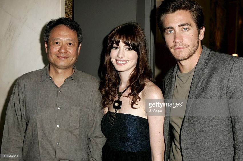
Compact Deep Aggregation for Set Retrieval                                                                                              9

Table 1: Distribution of faces per image in the ‘Celebrity                test dataset. The effects of varying the number of faces per
Together’ Dataset.                                                        set used for training are also studied. One randomly sam-
                                                                          pled face example per query identity is used to query the
       No. faces / image      2         3      4    5      >5
         No. images          113k      43k    19k   9k     10k
                                                                          dataset. The experiment is repeated 10 times using different
                                                                          face examples, and the nDCG scores are averaged.
Table 2: Distribution of annotations per image in the                     Test dataset synthesis. A base dataset with 64k face sets of
‘Celebrity Together’ Dataset.                                             2 faces each is synthesized, using only the face images of la-
   No. celeb / image        1     2      3     4      5      >5           belled identities in the Celebrity Together dataset. A random
     No. images            88k   89k    12k    3k   0.7k     0.3k         sample of 100 sets of 2 identities are used as queries, taking
                                                                          care that the two queried celebrities do appear together in
                                                                          some dataset face sets. To obtain four datasets of varying dif-
5 Experiments and results                                                 ficulty, 0, 1, 2 and 3 distractor faces per set are sampled from
                                                                          the unlabelled face images in Celebrity Together Dataset,
In this section we investigate four aspects: first, in Sec. 5.1
                                                                          taking care to include only true distractor people, i.e. people
we study the performance of different models (SetNet and
                                                                          who are not in the list of labelled identities in the Celebrity
baselines) as the number of faces per image in the dataset
                                                                          Together dataset. Therefore, all four datasets contain the same
is increased. Second, we compare the performance of Set-
                                                                          number of face sets (64k) but have a different number of faces
Net and the best baseline model on the real-world Celebrity
                                                                          per set, ranging from 2 to 5. Importantly, by construction, the
Together dataset in Sec. 5.2. Third, the trade-off between
                                                                          relevance of each set to each query is the same across all four
time complexity and set retrieval quality is investigated in
                                                                          datasets, which makes the performance numbers comparable
Sec. 5.3. Fourth, in Sec. 5.4, we demonstrate that SetNet
                                                                          across them.
learns to increase the descriptor orthogonality, which is good
for aggregation.                                                          Methods. The SetNet models are trained as described in
    Note, in all the experiments, there is no overlap between             Sec. 3.4, where the suffix ‘-2’ or ‘-3’ denotes whether 2- or
the query identities used for testing and the identities used             3-element sets are used during training. For SetNet, the op-
for training the network, as the VGG Face Dataset (Parkhi                 tional suffix ‘+W’ means that the set descriptors are whitened.
et al., 2015) (used for testing, e.g. for forming the Celebrity           For example, SetNet-2+W is a model trained with 2-element
Together dataset) and the VGGFace2 Dataset (Cao et al.,                   sets and whitening. Whereas for baselines, ‘+W’ indicates
2018) (used for training) share no common identities.                     whether the face descriptors have been whitened and L2-
Evaluation protocol. We use Normalized Discounted Cu-                     normalized before aggregation. We further investigate the
mulative Gain (Järvelin and Kekäläinen, 2002) (nDCG) to                effect of performing whitening after aggregation for the base-
evaluate set retrieval performance, as it can measure how well            lines, indicated as ‘+W (W after agg.)’. In this test, both
images containing all the query identities and also subsets of            SetNet and the baseline use ResNet-50 with 128-D feature
the queries are retrieved. For this measurement, images have              output as the feature extractor network.
different relevance, not just a binary positive/negative label;               Baselines follow the same naming convention, where
the relevance of an image is equal to the number of query                 the architectural difference from the SetNet is that the ag-
identities it contains. We report nDCG@10 and nDCG@30,                    gregator block is replaced with average-pooling followed
where nDCG@N is the nDCG for the ranked list cropped                      by L2-normalization, as shown in Fig. 2 (i.e. they use the
at the top N retrievals. nDCG is computed as the ratio be-                same feature extractor network, data augmentation, optional
tween DCG and the ideal DCG computed on the ground-truth                  whitening, etc.). The baselines are trained in the same man-
ranking, where DCG is defined as:                                         ner as SetNet. The exceptions are Baseline and Baseline+W,
              N
                                                                          which simply use the feature extractor network with average-
DCG@N = ∑ (2rel(i) − 1)/ log2 (i + 1)                               (3)   pooling, but no training. It is important to note that train-
             i=1                                                          ing the modified ResNet-50 and SENet-50 networks on the
where rel(i) denotes the relevance of the ith retrieved im-               VGGFace2 dataset (Cao et al., 2018) provides very strong
age. nDCGs are written as percentages, so the scores range                baselines (referred to as Baseline). Although the objective
between 0 and 100.                                                        of this paper is not face classification, to demonstrate the
                                                                          performance of this baseline network, we test it on the public
                                                                          IARPA Janus Benchmark A (IJB-A dataset) (Klare et al.,
5.1 Stress test                                                           2015). Specifically, we follow the same test procedure for
                                                                          the 1:N Identification task described in (Cao et al., 2018).
In this test, we aim to investigate how different models per-             In terms of the true positive identification rate (TPIR), the
form with increasing number of faces per set (image) in the               ResNet-50 128-D network achieves 0.975, 0.993 and 0.994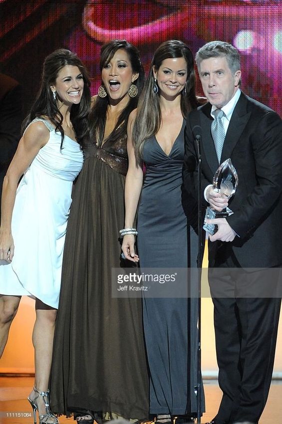
10                                                                                          Y. Zhong, R. Arandjelović and A. Zisserman

for the top 1, 5 and 10 ranking respectively, which is on par        Table 3: Number of images and faces in the test dataset.
with the state-of-the-art networks in (Cao et al., 2018).            The test dataset consists of the Celebrity Together dataset
    For reference, an upper bound performance (Descriptor-           and distractor images from the MS-Celeb-1M dataset (Guo
per-element, see Sec. 5.3 for details) is also reported, where       et al., 2016).
no aggregation is performed and all descriptors for all ele-
                                                                                                           Distractors
ments are stored.                                                                    Celebrity Together
                                                                                                          from MS1M
                                                                                                                          Total
Results. From the results in Fig. 5 it is clear that SetNet-2+W            Images           194k             355k        549k
and SetNet-3+W outperform all baselines. As Fig. 6 shows,                  Faces            546k              1M         1546k
nDCG@30 generally follows a similar trend to nDCG@10:
SetNet outperforms all the baselines by a large margin and,          sampled from the MS-Celeb-1M Dataset (Guo et al., 2016),
moreover, the gap increases as the number of elements per            as before taking care to include only true distractor people.
set increases. As expected, the performance of all models            The sampled distractor sets are constructed such that the
decreases as the number of elements per set increases due to         number of faces per set follows the same distribution as in
larger cross-element interference. However, SetNet+W de-             the Celebrity Together dataset. The statistics of the resultant
teriorates more gracefully (the margin between it and the            test dataset are shown in Table 3. There are 1000 test queries,
baselines increases), demonstrating that our training makes          formed by randomly sampling 500 queries containing two
SetNet learn representations which minimise the interference         celebrities and 500 queries containing three celebrities, under
between elements. The set training is beneficial for all ar-         the restriction that the queried celebrities do appear together
chitectures, including SetNet and baselines, as models with          in some dataset images.
suffixes ‘-2’ and ‘-3’ (set training) achieve better results than
those without (no set training).                                     Experimental setup and baseline. In this test we consider
                                                                     two scenarios: first, where only one face example is available
Whitening improves the performance for all architectures
                                                                     for each query identity, and second, where three face exam-
when there are more than 2 elements per set, regardless
                                                                     ples per query identity are available. In the second scenario,
whether the whitening is applied before or after the aggre-
                                                                     for each query identity, three face descriptors are extracted
gation. This is a somewhat surprising result since adding
                                                                     and aggregated to form a single enhanced descriptor which
whitening only happens after the network is trained. How-
                                                                     is then used to query the dataset.
ever, using whitening is common in the retrieval community
as it is usually found to be very helpful (Arandjelović and              In both scenarios the experiment is repeated 10 times
Zisserman, 2013; Jégou and Chum, 2012), but has also been           using different face examples for each query identity, and
used recently to improve CNN representations (Radenović             the nDCG score is averaged. The best baseline from the
et al., 2016; Sun et al., 2017). Radenović et al. (2016) train a    stress test (Sec. 5.1) Baseline-2+W (modified ResNet with
discriminative version of whitening for retrieval, while Sun         average-pooling), is used as the main comparison method.
et al. (2017) reduce feature correlations for pedestrian re-         Moreover, we explore three additional variations of the base-
trieval by formulating the SVD as a CNN layer. It is likely          line: (i) average-pooling the L2 normalized features before
that whitening before aggregation is beneficial also because         (rather than after) the final FC layer; (ii) (‘Baseline-GM’),
it makes descriptors more orthogonal to each other, which            replacing the average-pooling with generalized mean pool-
                                                                                                 1
helps to reduce the amount of information lost by aggrega-           ing, g(p) = 1n ∑nk=1 |xk | p p , (Radenović et al., 2018) where
tion. However, SetNet gains much less from whitening, which          the learnable parameter p is a scalar shared across all feature
may indicate that it learns to produce more orthogonal face          dimensions; and (iii) (‘Baseline-GM’ (p per dim.)), replacing
descriptors. This claim is investigated further in Sec. 5.4.         the average-pooling with generalized mean pooling where
    It is also important to note that, as illustrated by Fig. 6b,    the learnable parameter p is a vector with one value per di-
the cardinality of the sets used for training does not affect the    mension. Following (Radenović et al., 2018), the learnable
performance much, regardless of the architecture. Therefore,         parameter p is initialized to 3 for (ii) and to a vector of 3’s
training with a set size of 2 or 3 is sufficient to learn good set   for (iii). All three variations are trained with 2 elements per
representations which generalize to larger sets.                     set. The learnt p for (ii) is about 1.43. For (iii), the elements
                                                                     in the learnt p have various values mostly between 1.3 and
                                                                     1.5. Note that for (ii) and (iii), whitening happens after the
5.2 Evaluating on the Celebrity Together dataset                     aggregation due to the restriction of the non-negative values
                                                                     in the descriptors.
Here we evaluate the SetNet performance on the full Celebrity        Results. Table 4 shows that SetNets outperform the best base-
Together dataset.                                                    line for all performance measures by a large margin, across
Test dataset. The dataset is described in Sec. 4. To increase        different feature extractors (i.e. ResNet and SENet) and dif-
the retrieval difficulty, random 355k distractor images are          ferent feature dimensions (i.e. 128 and 256). The boost is
Compact Deep Aggregation for Set Retrieval 11
Scoring model 2/set 3/set 4/set 5/set
Baseline 66.3 38.8 23.7 17.5
Baseline-2 65.8 39.7 25.6 19.0
Baseline-3 65.9 39.4 24.8 18.4
SetNet 71.1 55.1 43.2 34.9
SetNet-2 71.0 57.7 44.6 36.9
SetNet-3 71.9 57.9 44.7 37.0
Baseline + W 62.3 42.3 30.8 23.3
Baseline-2 + W 62.3 44.1 32.6 25.7
Baseline-3 + W 62.1 44.0 32.3 25.6
Baseline-3 + W (W after agg.) 62.2 44.0 32.2 25.6
SetNet + W 71.2 57.5 45.7 37.8
SetNet-2 + W 71.3 59.5 47.0 39.3
SetNet-3 + W 71.8 59.8 47.1 39.3
Desc-per-element 72.4 69.4 67.1 65.3
(b)
(a)
Fig. 5: Stress test comparison of nDCG@10 of different models. There are 100 query sets, each with two identities. (a)
nDCG@10 for different number of elements (faces) per set (image) in the test dataset. (b) Table of nDCG@10 of stress test.
Columns corresponds to the four different test datasets defined by the number of elements (faces) per set.
Scoring model 2/set 3/set 4/set 5/set
Baseline 55.5 35.5 23.0 17.6
Baseline-2 55.4 36.3 24.6 18.8
Baseline-3 55.3 35.9 23.9 18.3
SetNet 61.1 49.2 39.1 32.2
SetNet-2 61.6 51.1 40.9 34.1
SetNet-3 61.5 51.2 41.0 34.2
Baseline + W 55.2 39.5 29.4 22.9
Baseline-2 + W 55.3 41.1 31.1 25.1
Baseline-3 + W 55.2 41.0 30.9 25.0
Baseline-3 + W (W after agg.) 55.2 41.0 30.9 25.0
SetNet + W 61.4 50.5 40.7 34.5
SetNet-2 + W 61.6 52.1 42.4 35.9
SetNet-3 + W 61.2 52.2 42.5 36.0
Desc-per-element 63.9 61.7 60.4 59.3
(b)
(a)
Fig. 6: Stress test comparison of nDCG@30 of different models. Columns corresponds to the four different test datasets
defined by the number of elements (faces) per set.
particularly impressive when ResNet with 128-D output is 2+W by the generalized mean with a learnable parameter
used and only one face example is available for each query p. In practice, we find that using a shared value of p for
identity, where Baseline-2+W is beaten by 9.1% and 10.0% all dimensions of the descriptors results in the best baseline
at nDCG@10 and nDCG@30 respectively. As we can see, model i.e. Baseline-GM-2+W. Although the baseline method
performing the average-pooling before the FC layer in the is improved by a better (and learnable) mean computation
feature extractor brings a marginal increase in the perfor- method, the gap between the baseline models and SetNet is
mance for the Baseline-2+W. A slightly larger enhancement still significant.
is achieved by replacing the average-pooling in Baseline-12 Y. Zhong, R. Arandjelović and A. Zisserman
Table 4: Set retrieval performance on the test set. De is the output feature dimension of the feature extractor CNN, and D is
the dimension of the output feature dimension of SetNet. Q is the number of identities in the query. There are 500 queries with
Q = 2, and 500 with Q = 3. Nex is the number of available face examples for each identity. Nqd is the number of descriptors
actually used for querying.
Scoring model Feature De D Nqd Scenario 1: Nex = 1 Scenario 2: Nex = 3
extractor nDCG@10 nDCG@30 nDCG@10 nDCG@30
Baseline-2 + W ResNet 128 - Q 50.0 49.4 56.6 56.0
Baseline-2 + W (agg. before FC) ResNet 128 - Q 50.2 49.5 56.6 56.0
Baseline-GM-2 + W ResNet 128 - Q 51.0 50.6 57.2 56.9
Baseline-GM-2 + W (p per dim.) ResNet 128 - Q 50.9 50.4 57.0 56.8
SetNet-3 + W ResNet 128 128 Q 59.1 59.4 63.8 64.1
SetNet-3 + W w/ query agg. ResNet 128 128 1 58.7 59.4 62.9 64.1
Baseline-2 + W SENet 128 - Q 52.9 52.5 59.6 59.5
SetNet-3 + W SENet 128 128 Q 59.5 59.5 63.7 64.5
SetNet-3 + W w/ query agg. SENet 128 128 1 59.1 59.5 63.4 64.0
Baseline-2 + W ResNet 256 - Q 56.8 57.8 62.5 64.2
SetNet-3 + W ResNet 256 256 Q 61.2 62.6 66.0 68.9
SetNet-3 + W w/ query agg. ResNet 256 256 1 60.3 62.4 65.1 68.8
Baseline-2 + W SENet 256 - Q 58.2 60.8 64.2 66.2
SetNet-3 + W SENet 256 256 Q 62.6 64.8 67.3 70.1
SetNet-3 + W w/ query agg. SENet 256 256 1 61.9 64.5 66.3 69.6
Similar improvement appears for SENet-based SetNet: next section, this drop can be nullified by re-ranking, making
6.6% at nDCG@10 and 7% at nDCG@30. When a feature di- query aggregation an attractive method due to its efficiency.
mension of 256 is used, we also observe that SetNet-3+W out- In the second scenario, apart from aggregating the query face
performs Baseline-2+W by a significant amount, e.g. 4.4% descriptors, we also investigated other ways of making use
at nDCG@10 on both ResNet and SENet. Note that the gap of multiple face examples per query, including scoring the
between the baseline and SetNet is smaller when we use dataset images with each face example separately followed
256-D set-level descriptors rather than 128-D. This indicates by merging the scores for each image under some combi-
that the superiority of SetNet is more obvious with lower nation rules (e.g. mean, max, etc.). However, it turns out
dimensionality. The improvement is also significant for the that simply aggregating the face descriptors for each query
second scenario where three face examples are available for identity achieves the best performance and, moreover, it is
each query identity. For example, an improvement of 7.2% the most efficient method as it adds almost no computational
and 8.1% over the baseline is observed on ResNet with 128- cost to the single-face-example scenario.
D output, and 4.1% and 5% on SENet. We can also conclude
that SENet achieves better results than ResNet as it produces
better face descriptors. In general, the results demonstrate 5.3 Efficient set retrieval
that our trained aggregation method is indeed beneficial since
it is designed and trained end-to-end exactly for the task in Our SetNet approach stores a single descriptor-per-set mak-
hand. Fig. 1 shows the top 3 retrieved images out of 549k ing it very fast though with potentially sacrificed accuracy.
images for two examples queries using SetNet (images are This section introduces some alternatives and evaluates trade-
cropped for better viewing). offs between set retrieval quality and retrieval speed. To
Query aggregation. We also investigate a more efficient evaluate computational efficiency formally with the big-O
method to query the database for multiple identities. Namely, notation, let Q, F and N be the number of query identities,
we aggregate the descriptors of all the query identities us- average number of faces per dataset image, and the number
ing SetNet to produce a single descriptor which represents of dataset images, respectively, and let the face descriptor be
all query identities, and query with this single descriptor. D-dimensional. Recall that our SetNet produces a compact
In other words, we treat all the query images as a set, and set representation which is also D-dimensional, and D = 128
then obtain a set-level query descriptor using SetNet. In the or 256.
second scenario, when three face examples are available for Descriptor-per-set (SetNet). Storing a single descriptor per
each query identity, all of the descriptors are simply fed to set is very computationally efficient as ranking only requires
SetNet to compute a single descriptor. With this query rep- computing a scalar product between Q query D-dimensional
resentation we obtain a slightly lower nDCG@10 compared descriptors and each of the N dataset descriptors, passing
to the original method shown in Table 4 (62.9 vs 63.8), and them through a logistic function, followed by scoring the
the same nDCG@30 (64.1). However, as will be seen in the images by the sum of similarity scores, making this stepCompact Deep Aggregation for Set Retrieval 13
O(NQD). For the more efficient query aggregation where but pre-tagging is very fast in practice as querying can be
only one query descriptor is used to represent all the query implemented efficiently using an inverted index.
identities, this step is even faster with O(ND). Sorting the Experimental setup. The performance is evaluated on the
scores is O(N log N). Total memory requirements are O(ND). 1000 test queries and on the same full dataset with distractors
Descriptor-per-element. Set retrieval can also be performed as in Sec. 5.2. Nr is varied in this experiment to demonstrate
by storing all element descriptors, requiring O(NFD) mem- the trade-off between accuracy and retrieval speed. Here,
ory. Assuming there is no need for handling strange (e.g. there is one available face example for each identity, Nex = 1.
Photoshopped) images, each query identity can be portrayed For the descriptor-per-element and pre-tagging methods, we
at most once in an image, and each face can only corre- use the Baseline + W features.
spond to a single query identity. An image can be scored Speed test implementation. The retrieval speed is measured
by obtaining all Q × F pairs of (query-identity, image-face) as the mean over all 1000 test query sets. The test is imple-
scores and finding the optimal assignment by considering mented in Matlab, and the measurements are carried out on a
it as a maximal weighted matching problem in a bipartite Xeon E5-2667 v2/3.30GHz, with only a single thread.
graph. Instead of solving the problem using the Hungarian
algorithm which has computational complexity that is cu-
5.3.1 Results
bic in the number of faces and is thus prohibitively slow,
we use a greedy matching approach. Namely, all (query- Table 5 shows set retrieval results for the various methods
identity, image-face) matches are considered in decreasing together with the time it takes to execute a set query. The full
order of similarity and added to the list of accepted matches descriptor-per-element approach is the most accurate one,
if neither of the query person nor the image face have been but also prohibitively slow for most uses, taking more than
added already. The complexity of this greedy approach is 6 seconds to execute a query using 128-D descriptors (and
O(QF log(QF)) per image. Therefore, the total computa- 8 seconds for 256-D.) The descriptor-per-set (i.e. SetNet)
tional complexity is O(NQFD + NQF log(QF) + N log N). approach with query aggregation is blazingly fast with only
For our problem, we do not find any loss in retrieval per- 0.01s per query using one descriptor to represent all query
formance compared to optimal matching, while being 7× identities, but sacrifices retrieval quality to achieve this speed.
faster. However, taking the 128-D descriptor as an example, using
Combinations by re-ranking. Borrowing ideas again from SetNet for initial ranking followed by re-ranking achieves
image retrieval (Philbin et al., 2007; Sivic and Zisserman, good results without a significant speed hit – the accuracy
2003), it is possible to combine the speed benefits of the almost reaches that of the full slow descriptor-per-element
faster methods with the accuracy of the slow descriptor-per- (e.g. the gap is 0.3% for ResNet and 0.8% for SENet at
element method by using the former for initial ranking, and nDCG@30), while being more than 35× faster. A even larger
the latter to re-rank the top Nr results. The computational speed gain is observed using 256-D descriptor, namely about
complexity is then equal to that of the fast method of choice, 45× faster than the desc-per-element method. Furthermore,
plus O(Nr QFD + Nr QF log(QF) + Nr log Nr ). by combining desc-per-set and desc-per-element it is possible
to choose the trade-off between speed and retrieval quality, as
Pre-tagging. A fast but naive approach to set retrieval is to
appropriate for specific use cases. For a task where speed is
pre-tag all the dataset images offline with a closed-world of
crucial, desc-per-set can be used with few re-ranking images
known identities by deeming a person to appear in the image
(e.g. 100) to obtain a 212× speedup over the most accurate
if the score is larger than a threshold. Set retrieval is then per-
method (desc-per-element). For an accuracy-critical task,
formed by ranking images based on the intersection between
it is possible to re-rank more images while maintaining a
the query and image tags. Pre-tagging seems straightforward,
reasonable speed.
however, it suffers from two large limitations; first, it is very
constrained as it only supports querying for a fixed set of Baselines. The best baseline method Baseline-GM-2+W is
identities which has to be predetermined at the offline tag- inferior to our proposed SetNet even when combined with
ging stage. Second, it relies on making hard decisions when re-ranking. This is mainly because the initial ranking using
assigning an identity to a face, which is expected to perform Baseline-GM-2+W does not have a large enough recall – it
badly, especially in terms of recall. Note to obtain high preci- does not retrieve a sufficient number of target images in the
sion (i.e. correct) results for tagging, 10 face examples are top 2000 ranks, so re-ranking is not able to reach the SetNet
used for making the decision on whether each predetermined performance.
identity is in the database images. Thus tagging is a some- Pre-tagging. Pre-tagging achieves better results than desc-
what unfair baseline as all the other methods operate in a per-set using SetNet descriptors without re-ranking. This is
more realistic scenario of only having one to three examples reasonable as pre-tagging should be categorized into the desc-
available. The computational complexity is O(NQ + N log N) per-element method, i.e. it performs offline face recognitionYou can also read