Comparing dominance of tennis' big three via multiple-output Bayesian quantile regression models
←
→
Page content transcription
If your browser does not render page correctly, please read the page content below
Comparing dominance of tennis’ big three via
                                           multiple-output Bayesian quantile regression models
                                                                                   Bruno Santos∗
arXiv:2111.05631v1 [stat.AP] 10 Nov 2021

                                                                               University of Kent

                                                                                       Abstract

                                                      Tennis has seen a myriad of great male tennis players throughout its his-
                                                  tory and we are often interested in the discussion of who is/was the greatest
                                                  player of all time. While we do not try to answer this question here, we delve
                                                  into comparing some key statistics related to dominance over their opponents for
                                                  the male players with the most Grand Slam titles, currently: Djokovic, Federer
                                                  and Nadal, in alphabetical order. Here we consider the minutes played and the
                                                  relative points in each of their completed matches, as a measure of dominance
                                                  against other players. We consider important covariates such as surface, win
                                                  or loss, type of tournament and whether their opponent was a top 20 ranked
                                                  player in the world or not, to create a more complete comparison of their per-
                                                  formance. We consider a Bayesian quantile regression model for multiple-output
                                                  response variables to take into account the dependence between minutes and rel-
                                                  ative points won. This approach is compelling since we do not need to choose a
                                                  probability distribution for the joint probability distribution of our response vari-
                                                  able. Our results agree with the common intuition of Nadal’s superiority in clay
                                                  courts, Federer’s superiority in grass courts and Djokovic’s superiority in hard
                                                  courts given their success in each of these surfaces; though Nadal’s dominance
                                                  in clay court games is unique. Federer shows his dominance regarding minutes
                                                  spent in the court in wins, while Djokovic takes the edge when considering the
                                                  dimension of relative points won, for most of the comparisons. While minutes
                                                  can be directly connected to style of play, the relative points dimension could
                                                  express more directly different levels of advantage over their opponent, in which
                                                  Djokovic seems to be the overall leader in this analysis.
                                            ∗
                                                e-mail: b.santos@kent.ac.uk

                                                                                           1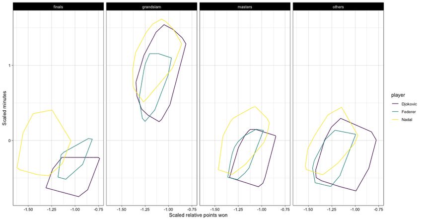
1     Introduction
Between the Wimbledon tournament in 2003 and the US Open in 2021, there were
74 Grand Slam tournaments played in competitive tennis. These tournaments are the
most prestigious and the most important tournaments in tennis, given their points and
money rewarded to players. In the men’s side, in 60 of those 74 tournaments the winner
of the tournament was in a small group of three very special players, also known in
some media outlets as the ”Big Three”: Novak Djokovic, Roger Federer and Rafael
Nadal. This is a quite long period of domination in the sport, where these three great
players won more than 80% of their matches and have amassed almost more than 3000
wins, with Djokovic just the one short of 1000 careers wins, with 978 at the time of
writing this manuscript. This is certainly a measure of dominance of these players
against all the others in the Association of Tennis Professionals (ATP) tour. Given
this dominance over the years, an interesting question could be posed as to find out
who is the more dominant among them.
    There is certainly a great deal of debate if either one of these great three can be
considered as the Greatest of All Time (GOAT) in the men’s side. In fact, Baker and
McHale (2014) studied the games of the Open Era and concluded that Roger Federer
was a good choice for the GOAT title with all the available information regarding games
played up until 2014. This is definitely an interesting discussion, but when one tries to
answer this kind of question, it needs to use information or variables available for all
players. In this case, one possible approach is try to estimate the probability of winning
each match given the opponent. This could give an estimate of strength for each player,
which could then be compared across different periods of tennis. The problem with this
type of method is that it disregards possible differences between players from different
eras, as far as conditioning, training regimes, ease (or difficulty) of travelling, level of
play across the ATP tour, among others. The evolution of the game itself, for instance,
regarding the material being used in the rackets could certainly have a difference in
how these players have performed over time. For this reason, we avoid the comparison
between players of different eras.
    Other modelling efforts with tennis data have looked at different questions as well.
Knottenbelt et al. (2012) considered a hierarchical Markov model to explain the prob-
ability of a player winning a match. Still on estimating this probability of winning a
match, McHale and Morton (2011) examined a Bradley-Terry type of model, taking
into account the surfaces as well to forecast the final result; Klaassen and Magnus

                                             2
(2003) proposed a method to update the probabilities of winning during the match as
well and not just at the beginning. del Corral and Prieto-Rodriguez (2010) used the
difference of rankings to predict the outcomes of matches in Grand Slams. Gorgi et al.
(2019) considered a high dimensional dynamic model with player and surface specific
parameters that was able to give better forecasts and it could be used to rank players
as well.
Here in this paper we focus our attention to data only pertaining to these three great
players, who currently lead the grand slam titles list and are tied with 20 wins apiece:
Djokovic, Federer and Nadal. The reason for not to include data from different players
is the assumption that due to their extraordinary career path, their variation might
not be explained by standards of regular players in the tour. For example, the model
proposed by Gorgi et al. (2019) predicts that Nadal had a 60% probability of winning a
match against Federer in a clay court game in February of 2017, which sounds slightly
conservative given their record in clay courts games with 13 wins to Nadal and only 2
to Federer at that point. This is not an attempt of dismissing their work, but rather
an indication that using other players information to get a possible baseline estimate
and adding player specific components to explain these player abilities might not be
appropriate for the big three.
The variables considered in this analysis were chosen to approximate the idea of
dominance or superiority between players during a tennis match. While one can agree
that a quick match is not equivalent to being an ”easy” win for one of the sides
or a dominant win, we often observe that an easier match for a specific player will
take less time on the clock in comparison with a tighter match. Therefore, one can
think of duration of the match as a necessary condition, but not a sufficient one to
approximate dominance of a particular match. Also, when one considers each single
point separately, we could think that every player will try to win every point, even
though sometimes their effort might not be the same at all points. How many points a
player wins against another one relatively could give an idea of superiority in this sense.
For instance, Klaassen and Magnus (2001) posed the question whether points in tennis
are independent and identically distributed and found out that the weaker a player is
the stronger would be the effect contrary to their question. Even though, winning more
points is not necessary a condition for winning the match, we believe that the relative
points won does approximate the notion of dominance within a match. For example,
we could use points won divided by points lost in a given match to measure this effect.
3With the aim to compare the dominance of these players against their opponents, we
consider then minutes of each match for these players and relative points won as our
response variable. Assuming that these variables are correlated, modelling them jointly
certainly will bring more information.
In our modelling analysis, we consider Bayesian quantile regression models for mul-
tiple output response variables, in order to consider the information in both variables
in the discussion of our results. The reason for this choice is the possibility of mod-
elling these variables jointly, therefore using their correlation to build a more complete
picture of their variation, but without assuming any probability distribution. Quantile
regression models have been used for a number of applications since their inception
by Koenker and Bassett (1978) and have shown a great value to explain conditional
quantiles, with flexibility to approximate these measures even without assuming any
probability distribution for the response variable. A multivariate proposal was dis-
cussed by Hallin et al. (2010), where a directional approach is taken to estimate each
quantile and a connection between quantile regions and depth regions was made. We
consider the results of Santos and Kneib (2020), where the authors considered the
problem of estimating several quantiles of interest and proposed a method to obtain
noncrossing quantiles in this multivariate setting. Nevertheless, here we focus in just
one quantile, τ = 0.25, in order to have a more central quantile region to compare the
performance of these players given the different covariates. Also, in our analysis the
results were rather similar considering other values for τ .
We organize this manuscript in the following manner. In the next section, we
present the data set and its details regarding filters used to select the observations
considered in the modelling part. In Section 3, we give a brief introduction to Bayesian
quantile regression models for multiple-output variables, as proposed by Santos and
Kneib (2020). In the following section, we present our main results, where we compare
the outputs of the model for different combinations of the covariates. We finish this
manuscript with our final comments on Section 5.
2 Data set
We consider the data set organized by Jeff Sackman and available at the following
repository: https://github.com/JeffSackmann/tennis_atp. We use all matches
between 1998, the year where Federer started playing professionally, and until the US
4Open of 2020. For our analysis, we are interested only in the matches, where one of
the players is either Roger Federer, Novak Djokovic or Rafael Nadal, so we filter their
games only. We do not select matches where one of the players withdrawn or did not
complete the match because of an injury, therefore only completed matches are taken
into account. We also removed matches from Davis Cup and the Olympic Games.
Moreover, because one of the variables of interest is the surface and since the number
of games on carpet was very small for these players, since they ATP stopped using this
material in 2009, we also removed matches played on that surface. After this selection
process, we have a total of 3,653 observations.
We are specially interested in variables regarding minutes played and relative points
won in each match. Although minutes could be directly affected by the differences in
how each player prepares for each point played, as far as how much time they take
in between points, but also in their approach throughout the match, we still consider
that this information could be connected to how it was easily won by one of the players
(not necessarily Djokovic, Federer or Nadal) or how hard the match was. In this case,
less minutes in court could be linked to a greater dominance, while more minutes could
be associated with less dominance or a closer match. Nevertheless, this needs to be
controlled by the surface, since clay courts games usually take longer to finish than
those played on grass or hard courts, for instance. Moreover, grand slam tournaments
are played as best of 5 sets, instead of best of 3, which is the case for most of the
tournaments. Therefore, we need to take into account the tournament type as well.
In Figure 1, we can see the scatter plot between these two variables. One is able to
see that longest matches are closer to the value 1.0 of relative points won. In fact, the
longest match in the data set is related to the Australian Open final between Djokovic
and Nadal in 2012, where they battled for almost 6 hours. In this case, this match is
duplicated at the highest value for the y axis, where the difference in x axis shows the
two values for relative points for each player; by definition, these values are symmetrical
around 1. For this particular match, Djokovic won the match and also around 9% more
points than Nadal, which puts relative points won close to the value 1.09.
We can also note that matches, where these players had a bigger (or smaller)
value for relative points won, had a lower minutes value, which seems appropriate.
If one of the players wins (or loses) the majority of the points, this match should
finish in fewer minutes. Though this is certainly not a sufficient condition for faster
matches. It is important to emphasise that points themselves are not exactly connected
5Figure 1: Scatter plot between relative points won and minutes played for all com-
pleted matches for Djokovic, Federer and Nadal.
to winning or losing, since players need to win games, in order to win sets, in order to
win the match. There is surely a connection between these outcomes, but this is not
exact. For instance, for these three great players and their completed matches shown
in Figure 1, in around 10% of their losses they still managed to win more points than
their opponent throughout the match. This number is around 5% if we consider all
matches in this period in the ATP tour. Due to this higher performance even in losses,
in comparison with the rest of the ATP tour, we believe it is worth considering as one
of our covariates, whether the match was won or lost by the big three. Because tennis
is a sport where a loss is equivalent to an elimination of the tournament, with the
exception of tournaments like Finals, it is intriguing to compare their performance in
these different types of games.
Given the different types of numbers of players involved and even participation of
top players, we split the tournaments in 4 different types: Grand Slam, Masters, Finals
and others. Grand Slams are the most important and the most prestigious tournaments
and they are played as a best of five sets format. Therefore, it is important that they
are on their own category. Masters tournaments are currently known as Masters 1000
and there are nine tournaments of this level throughout the year, being played in
all different surfaces and continents around the world. Finals is just one tournament
6played with the best 8 players of each year. They are played in a different structure,
in a round robin format, where players are divided in two groups and the best two
of each group are headed to the semifinals, after all playing against each other inside
the group. Besides these tournaments, we consider all other tournaments in the same
category. § If we want to discuss dominance against other players, it is important to try
to measure how each one of these three great tennis players fared against different type
of competition. Besides considering the effects for surface and types of tournaments,
we split their matches against top 20 players in the world rankings and other players.
This is to show how they contrast when facing a more challenging opponent, given by
a higher ranking, in comparison with games against players not so well ranked. This
is not an admission of easier games against opponents outside this interval, but rather
a remark about the high quality of play that tennis players must attain to reach a top
20 world ranking. When those players reach this level, one anticipates tight matches
and it is important to compare the performance of the big three against this level of
competition.
We could have used age as well as one of our covariates, but we decided to omit
that information given the rather amazing career path that each one of these players
took while ageing in a different manner than most players. For instance, Gorgi et al.
(2019) estimates that players on average reach their highest performance around age
of 25 years. While this is possibly true for most of the players, it might not hold true
to the big three. Federer and Nadal first achieved the number one rankings at the age
of 22 years old, while Djokovic reached the top at 24 years old. Between 2004 and
2020, they have been swapping this first position continuously, except for one year,
when Andy Murray finished the year as the best player in the planet. They are now
the oldest players ever to hold the number one ranking, with Federer currently leading
this category when he obtained the highest position in the ranking at the age of 36
years old. Given these circumstances, we decide to focus their comparisons taking into
consideration only other variables described here in this section.
3 Bayesian quantile regression for multiple output
response variables
Considering our two dimensional response variable, relative points won and minutes, we
would like to describe their joint variation as a function of all the variables described
7in the previous section. Given their variation presented in Figure 1, we would like
to study their conditional probability distribution, without assuming any probability
distribution at first. Taking that into consideration, we consider a Bayesian form
of the directional quantile regression model for multiple outputs proposed by Hallin
et al. (2010). We use the same approach proposed by Santos and Kneib (2020), where
an asymmetric Laplace distribution is considered in each direction of interest in the
likelihood of our model.
Regarding this model, we need to define a few quantities. First, let a directional
index be τ ∈ B k := {v ∈ Rk : 0 < ||v||2 < 1}, a collection of vectors encompassed in
the unit ball of Rk . We can split this directional index in two parts, τ = τ u, where
u ∈ S k−1 := {z ∈ Rk : ||z|| = 1}, represents the direction and τ ∈ (0, 1) the magnitude
of interest. Moreover, let let Γu be an arbitrary k ×(k −1) matrix of unit vectors, where
. 0
(u .. Γu ) establishes an orthonormal basis of Rk . Define Y u := u Y and Y ⊥ := Γu Y .
0
Therefore, for each direction we consider a mixture representation of the asymmetric
Laplace proposed by Kozumi and Kobayashi (2011), as the following
Yu |bτ , β τ , σ, v ∼ N (η u + θv, ψ 2 σV ),
vi ∼ Exp(σ), i = 1, . . . , n,
where θ = (1 − 2τ )/(τ (1 − τ )), ψ 2 = 2/(τ (1 − τ )), Exp(σ) denotes the exponential
distribution with mean σ, V = diag(v1 , . . . , vn ) and β τ contains a intercept. Our linear
predictor for this model is defined as
η u = Xβ τ + Yu⊥ bτ ,
where X is a n × p design matrix containing our covariates and an intercept.
Then one needs to define priors distributions for ξ = (bτ , β τ , σ) to complete the
specification of the model. For bτ , Guggisberg (2019) discusses its prior elicitation,
where the author relates this prior to the Tukey depth of the data. Combined with β τ ,
we use a multivariate normal distribution with mean 0 and a large variance for these
parameters for (bτ , β τ ). For σ, we consider an inverse gamma distribution as in Wald-
mann et al. (2013). Inference on the parameters is based on samples of the posterior
distribution obtained via Gibbs sampling and we refer to these previous references for
more details. Our estimates for each parameter will be defined as the posterior means,
namely (b̂τ , β̂ τ , σ̂).
8Given these parameters estimates, which are obtained for each direction u, we are
able to define an upper closed quantile halfspace
0 0 0
Hτ+u = Hτ+u (b̂τ , β̂ τ ) = {y ∈ Rk : u y ≥ b̂τ Γu y + x β̂ τ } (1)
and a lower open quantile halfspace switching ≥ for < in (1). Moreover, for fixed τ we
define the τ quantile region R(τ ) as
\
R(τ ) = Hτ+u . (2)
u∈S k−1
These quantile regions are important as we use them to study the effect of each pre-
dictor variable in the conditional distribution of Y . Hallin et al. (2010) showed that
this quantile region are equal to Tukey depth regions, which have been extensively
studied to describe the probability distribution of multivariate distributions. In our
case, we consider the boundary of these regions, also called quantile contours to make
the comparison between the results obtained by the three great players. Even though
Hallin and Šiman (2017) alert that severe assumptions are needed in order for these
quantities to be the depth contours of the conditional distribution of Y given X, we
follow Santos and Kneib (2020) and consider that these can be considered an averaged
version of the Tukey depth contour. We consider the same algorithm proposed by the
latter and in the next section we will use these quantile contours to make the compar-
isons between Djokovic, Federer and Nadal, conditional on the variables described in
Section 2.
4 Results
For our application, we estimate Bayesian quantile regression models for multiple out-
put as described in the previous section and show here the quantile contours for different
combinations of the covariates. We consider the data outlined in Section 2, where our
main interest lies in the bivariate response variable, relative points won and minutes.
Four our modelling purposes, we consider 180 directions defined uniformly in the
unit ball. We take τ = 0.25, so we can have a more central quantile region to compare
their results. We have tried other values for τ and the conclusions are quite similar.
For each direction, for each chain we consider a burn-in size of 10,000 and we run the
9chain to obtain 100,000 observations, keeping every 100th draw from this posterior.
We consider the following covariates for our model, with reference category denoted
inside the parenthesis. We use main effects to denote players (Federer - reference,
Djokovic, Nadal); win (no - reference, yes); surface (hard - reference, clay, grass);
tournament (others - reference, Grand Slam, Finals, Masters); top 20 (no - reference,
yes). Given our objective of comparing the three players, we add an interaction term
between player and all other covariates. Although we do not the equation here, the idea
is easy to follow, as we need to have a dummy variable for each one of the categories
that are not defined as the reference. Besides, there needs to be a coefficient for each
one of the interactions. In total, for this regression part of the model we are interested
in 24 parameters plus the coefficient related to the direction projection Yu⊥ . Therefore,
to avoid a long equation we decided to skip its definition here. We have to denote also
that each one of these parameters is attached to a direction and the visualisation (or
the analysis) is possible via the comparison of the quantile regions.
For each direction, we considered a transformation of the response variable to make
computations more stable. Instead of using each variable in their original scale, we
stardardized their value, i.e., we centered each variable by subtracting its mean and
divided by its standard deviation. In order to show the obtained quantile contours, we
still consider this range of variation, though one could also transform to the original
scale given how quantile are equivariant to monotone transformations. Because we
are considering the transformed values, we must always compare the variation among
the different quantile contours for the different players, instead of their actual values.
Moreover, in order to observe the effects of each covariate, we plot its respective quantile
contours for the three players, but we keep the values for all the other covariates at
their reference value. For instance, the reference value for variable win is no, then for
this reason the range of values in the x axis will be mostly negative. Likewise, we
reiterate that the differences among the different players and the different covariate
values is more important than the value itself.
We move to our conclusions first considering the quantiles contours that compare
their performances in wins and losses presented in Figure 2. In the dimension of time
in wins, there is a clearly advantage for Federer, as his quantile contours presents the
smallest values for that dimension. For the other variable, relative points won, for
either losses or wins, Djokovic has an advantage over the other two. When we compare
the quantile contours of Federer and Nadal, they have a quite similar structure, but
10Figure 2: Quantile contours to compare the performance between Djokovic, Federer
and Nadal in their losses and wins. For all other variables we consider their reference
value.
Nadal’s contour is moved upwards in the time dimension. In wins though, Nadal
shows a small advantage over Federer in the relative points won dimension. Another
interesting point in this comparison is how the correlation between these two variables
seems to be higher for wins rather than losses. In this case, for wins it is easier to see
that as the relative points won increases, the minutes variable decreases, which agrees
with a common intuition about the game: when these three win most of the points the
match will end more rapidly. The same cannot be said about losses.
When we consider the effect of playing against top 20 players in the ranking or not,
we can compare the quantile contours presented in Figure 3. A first look shows that in
the time dimensions for all three players there is a shift upwards when we compare their
performance against the best players in comparison with not so high ranked players.
Moreover, in the relative points won dimension, there is a shift to the left, meaning
that these games are possibly more difficult, or at least closer in this sense, against
high ranked players. Again, this would follow our common intuition about their results.
Furthermore, still in the relative points won perspective, while Djokovic seems to have
an advantage against lower ranked players, Federer presents a quantile region with less
variance and with the highest values equivalent to Djokovic highest values.
11Figure 3: Quantile contours to compare the performance between Djokovic, Federer
and Nadal in their matches against players in top 20 positions of the world rankings
or not. For all other variables we consider their reference value.
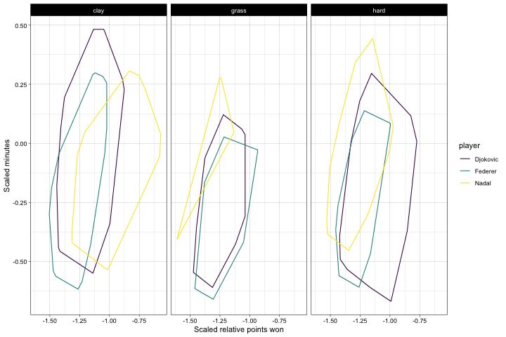
Figure 4: Quantile contours to compare the performance between Djokovic, Federer
and Nadal in their matches considering the three different surfaces. For all other
variables we consider their reference value.
12In the comparison about surfaces, which is shown in Figure 4, we have an interesting
expression of the dominance of each player in a different surface. First, only analysing
the relative points won dimension, Nadal is far superior in clay, Federer leads in grass
courts and Djokovic is ahead in hard courts. This is expected since Nadal is the possibly
the best ever player in clay courts, where he has 13 French Open titles, the Grand
Slam played in that surface. Meanwhile, Federer has the most titles in Wimbledon,
which is played in grass courts and Djokovic leads the titles in the Australian Open, a
hard court event. Both Federer and Djokovic have a good number of titles in the US
Open, another event in hard court, but that does not make their difference smaller. In
fact, Nadal is slight ahead of Federer in that direction. Regarding minutes spent on
court, Federer shows smaller values than the other in clay and grass court games. For
games played on hard courts, Djokovic does attain the smallest of the values in this
dimension on hard courts, though Federer’s quantile region is contained in a smaller
space, which indicates a smaller variation of values. Interestingly, when one compares
the different quantile regions across the surfaces, Nadal’s case in clay courts, seems to
be the most far off from the other. His quantile region is moved completely to the right
in comparison with the other. Djokovic dominance in hard courts is quite big too, but
for some directions his quantile region is not too distant from Federer region. This is
an evidence to describe that even though each one has an edge on a particular surface,
Nadal’s clay court dominance possibly is the biggest of them all.
Regarding the different tournament types, one can easily perceive the difference
between Grand Slam tournaments and the other tournaments in the minutes dimension,
displayed in Figure 5. All quantile regions from Grand Slam tournaments for the three
players are noticeably above the other tournaments. This is no surprise given the best
of five sets format for the more prestigious tournaments. Still on the time dimension,
Nadal appears to be the player with higher minutes on court, while Djokovic is the
one who gets the smallest values in his region. In the relative points won dimension,
Djokovic shows the highest values for all types of tournaments, with Nadal in second
in all types except the Finals. Notably, Nadal quantile region for this tournament is
rather different than the other players. In fact, Nadal has no titles in this type of
tournament, which could explain this result. Overall, one would give Djokovic the
acknowledment as the most dominant in all types of tournaments, when controlling
with the other variables.
13Figure 5: Quantile contours to compare the performance between Djokovic, Federer
and Nadal in their matches considering four different types of tournaments. For all
other variables we consider their reference value.
5 Concluding remarks
For this manuscript, we made an effort to discuss which one of the these three great
players of tennis, Djokovic, Federer and Nadal, is more dominant. We used the infor-
mation about their minutes and relative points won in each one of their matches and
considered some covariates, such as win or losses, surfaces, top 20 opponent or not and
type of tournament. By considering a Bayesian regression model for multiple output
response variables we were able to compare their results jointly regarding these two
response variables, without assuming a joint probability distribution for our response
variable. This presents a more flexible way of comparing this conditional probability
distributions of interest with less restrictions about their exact shape, for instance.
Conclusions about the results of each player were based on the comparison of their
quantile region conditional on the chosen covariates.
There are a few interesting results, which are worth mentioning given the plots
presented in the previous section. While each player showed some dominance in one
specific surface, Nadal’s superiority in clay court is simply above the others. His
unprecedented record of 13 French Open titles and many other titles in clay courts
14probably does support this result. Federer quickness in wins, with his quantile region
shifted downwards in comparison with the other two, is certainly meaningful. This
could be attributed perhaps to his playing style, since Nadal and Djokovic are known
to rely more heavily in their remarkable defensive skills. With the results presented
here, Djokovic should be considered the most dominant of the three. Specially, when
one considers the relative points won dimension, which seems to be a more powerful
quantity to measure this information. For this dimension, Djokovic is ahead in many
of the combination of covariates considered. This is possibly a testament to the several
accolades he has received during his accomplished career. He is, currently, the only
one between the three who has won each Grand Slam tournament at least twice and
also the only who won at least once all the Masters tournaments. This is certainly one
way of defining dominance.
This is possibly not the last comparison of these great players, but this application
was able to show some fascinating results for these great players. Though the measures
used here to describe dominance have their weaknesses, we believe they still give an
interesting approximation of superiority against their opponents. We hope that this
manuscript, where we used a different approach, not only regarding the modelling
technique, but also the chosen variables, leads to other stimulating discussions in this
area.
References
Baker, R.D., McHale, I.G.: (2014), A dynamic paired comparisons model: Who is the
greatest tennis player? European Journal of Operational Research 236, 677–684.
del Corral, J., Prieto-Rodriguez, J.: (2010), Are differences in ranks good predictors
for grand slam tennis matches? International Journal of Forecasting 26, 551–563,
sports Forecasting.
Gorgi, P., Koopman, S.J., Lit, R.: (2019), The analysis and forecasting of tennis
matches by using a high dimensional dynamic model. Journal of the Royal Statistical
Society: Series A (Statistics in Society) 182, 1393–1409.
Guggisberg, M.: (2019), A Bayesian Approach to Multiple-Output Quantile Regres-
sion. arXiv e-prints arXiv:1909.02623.
15Hallin, M., Paindaveine, D., Šiman, M.: (2010), Multivariate quantiles and multiple-
output regression quantiles: From l1 optimization to halfspace depth. The Annals of
Statistics 38, 635–669.
Hallin, M., Šiman, M.: (2017), Multiple-output quantile regression. In: Handbook
of quantile regression, edited by R. Koenker, V. Chernozhukov, X. He, L. Peng,
Chapman and Hall/CRC.
Klaassen, F.J., Magnus, J.R.: (2003), Forecasting the winner of a tennis match. Euro-
pean Journal of Operational Research 148, 257–267.
Klaassen, F.J.G.M., Magnus, J.R.: (2001), Are points in tennis independent and iden-
tically distributed? evidence from a dynamic binary panel data model. Journal of
the American Statistical Association 96, 500–509.
Knottenbelt, W.J., Spanias, D., Madurska, A.M.: (2012), A common-opponent
stochastic model for predicting the outcome of professional tennis matches. Com-
puters & Mathematics with Applications 64, 3820–3827.
Koenker, R., Bassett, G.: (1978), Regression quantiles. Econometrica 46, 33–50.
Kozumi, H., Kobayashi, G.: (2011), Gibbs sampling methods for Bayesian quantile
regression. Journal of Statistical Computation and Simulation 81, 1565–1578.
McHale, I., Morton, A.: (2011), A Badley-Terry type model for forecasting tennis
match results. International Journal of Forecasting 27, 619–630.
Santos, B., Kneib, T.: (2020), Noncrossing structured additive multiple-output
Bayesian quantile regression models. Statistics and Computing 97, 825.
Waldmann, E., Kneib, T., Yue, Y.R., Lang, S., Flexeder, C.: (2013), Bayesian semi-
parametric additive quantile regression. Statistical Modelling 13, 223–252.
16You can also read