Constrained-Differential-Kinematics-Decomposition-Based NMPC for Online Manipulator Control with Low Computational Costs
←
→
Page content transcription
If your browser does not render page correctly, please read the page content below

robotics
Article
Constrained-Differential-Kinematics-Decomposition-Based
NMPC for Online Manipulator Control with Low
Computational Costs
Jan Reinhold * , Henry Baumann                     and Thomas Meurer

                                         Automation and Control Group, Faculty of Engineering, Kiel University, Kaiserstraße 2, 24143 Kiel, Germany
                                         * Correspondence: janr@tf.uni-kiel.de; Tel.: +49-431-880-6121

                                         Abstract: Flexibility combined with the ability to consider external constraints comprises the main
                                         advantages of nonlinear model predictive control (NMPC). Applied as a motion controller, NMPC
                                         enables applications in varying and disturbed environments, but requires time-consuming compu-
                                         tations. Hence, given the full nonlinear multi-DOF robot model, a delay-free execution providing
                                         short control horizons at appropriate prediction horizons for accurate motions is not applicable in
                                         common use. This contribution introduces an approach that analyzes and decomposes the differential
                                         kinematics similar to the inverse kinematics method to assign Cartesian boundary conditions to
                                         specific systems of equations during the model building, reducing the online computational costs.
                                         The resulting fully constrained NMPC realizes the translational obstacle avoidance during trajectory
                                         tracking using a reduced model considering both joint and Cartesian constraints coupled with a
                                         Jacobian transposed controller performing the end-effector’s orientation correction. Apart from a safe
                                         distance from the obstacles, the presented approach does not lead to any limitations of the reachable
                                         workspace, and all degrees of freedom (DOFs) of the robot are used. The simulative evaluation in
                                         G AZEBO using the Stäubli TX2-90 commanded of ROS on a standard computer emphasizes the sig-
                                         nificantly lower online computational costs, accuracy analysis, and extended adaptability in obstacle
                                         avoidance, providing additional flexibility. An interpretation of the new concept is discussed for
                                         further use and extensions.
Citation: Reinhold, J.; Baumann, H.;
Meurer, T. Constrained-Differential-     Keywords: kinematic analysis; robotic differential model decomposition; nonlinear model predic-
Kinematics-Decomposition-Based           tive control (NMPC); controller couplings; joint and Cartesian space constraints; computing time
NMPC for Online Manipulator              reduction; accuracy analysis; trajectory tracking; obstacle avoidance
Control with Low Computational
Costs. Robotics 2023, 12, 7. https://
doi.org/10.3390/robotics12010007

Academic Editor: Raffaele Di             1. Introduction
Gregorio                                       Modern industry is in a constant state of change driven by the contemporary labor
Received: 15 November 2022
                                         market, the purchase demand, and the effective use of resources or machines [1]. Robots
Revised: 12 December 2022                are increasingly being used in process automation to carry out monotonous and strenuous
Accepted: 20 December 2022               work, also reducing the operating costs [2,3]. In addition, efficient image recognition and
Published: 3 January 2023                sensor fusion enable increasingly accurate recognition of the environment in the robot’s
                                         workspace [4]. Thus, using appropriate algorithms, robots can also be deployed in varying
                                         and disturbed environments to cover further fields of activity [5].
                                               One sector undergoing a tremendous transformation is agriculture, which motivates
Copyright: © 2023 by the authors.        this paper, but does not limit the scope of the presented approach. On the one hand, farmers,
Licensee MDPI, Basel, Switzerland.       industry, and governments need to keep the costs moderate, even in high-wage countries,
This article is an open access article   and on the other hand, consumers appreciate a sustainable and regional production [6].
distributed under the terms and          These requirements are not mutually exclusive, but this is a subject area that needs to be
conditions of the Creative Commons
                                         developed, among other fields of application [7]. In particular, image recognition has been
Attribution (CC BY) license (https://
                                         improved and adapted to specific agricultural problems in the last decade, allowing high-
creativecommons.org/licenses/by/
                                         quality recognition with many features in widely disturbed environments [8–10]. Precision
4.0/).

Robotics 2023, 12, 7. https://doi.org/10.3390/robotics12010007                                              https://www.mdpi.com/journal/robotics
Robotics 2023, 12, 7                                                                                              2 of 24

                       agriculture enables, e.g., mechanical weed removal without damaging the adjacent plants,
                       so that the use of pesticides can be reduced [11,12]. This usually requires equipment that is
                       dedicated to a specific application and is expensive to purchase and maintain. In contrast,
                       (industrial) robots are flexible and sustainable, as they are applicable for multiple applications
                       throughout the agricultural season, simply by using different end-effectors. However, for
                       the application in a distributed environment with multiple obstacles, trajectory planning
                       and control have to be accomplished almost delay-free. Achieving low computational costs
                       in optimal control using a robot with multiple degrees of freedom (DOFs) is addressed in
                       this work.
                             Motion control is used for the adaption of planned trajectories in the Cartesian or
                       joint space [13,14], which must subsequently be adjusted to a varying environment by means
                       of a closed control loop. In general, either a discrete or a continuous interpretation of the
                       workspace can be chosen. When choosing the discrete approach, the detected environment
                       is meshed [15], and the optimal path is planned along the resulting nodes and edges [16].
                       Here, the Dijkstra and A* algorithms [17], as well as sampling-based methods can be applied
                       with low computational cost to solve the planning task [18]. In general, inverse kinematics or
                       Jacobian inverse controllers with low computational costs are subsequently used for the
                       transformation into the joint space [19]. However, setting up the mesh is computational
                       expensive, so that a delay-free motion control is not possible in a highly varying environ-
                       ment [20,21]. Examples of continuous motion planning tools include CHOMP, STOMP,
                       and TrajOpt [22–24], which are commonly used. However, even though the computation
                       times are short, they are not optimized to be used iteratively for delay-free control [25].
                       In addition, learning-based methods are increasingly applied, especially to take the aging
                       of the robotic systems into account during motion control [26]. Using iterative learning
                       control [27], motions are repeated until the solution is within an acceptable range. However,
                       for motions in a varying environment, it is complicated to train these systems, as individual
                       movements have to be run several times with the same initial and terminal states [28]. If a
                       reference trajectory is known, the repetitive control approach can be added to be periodic
                       and address the initialization problem [29]. Furthermore, reinforcement learning is used to
                       improve the performance of the tracking controllers [30]. However, this paper presents a
                       model-based control scheme that adapts the motion based on the robot’s kinematic specifi-
                       cations. To realize a closed control loop, which iteratively considers varying environmental
                       constraints in the Cartesian space and robotic constraints in the joint space given by the
                       multi-DOF robot, nonlinear model predictive control (NMPC) is used [31]. As the dynamic
                       optimization has to be solved on a receding horizon, computational efficiency is an issue
                       for real-time application.
                             Two different time horizons have to be considered during the implementation of
                       NMPC [32,33]. The prediction horizon specifies how far the movements in the disturbed
                       environment are predicted. Governed by the sample size and the DOFs, the number of
                       decision variables is set, which determines the computational costs to solve the optimal
                       control problem (OCP) online [34]. Secondly, the control horizon, which is shorter than the
                       prediction horizon, describes a kind of buffer along which the robot executes the movements
                       of the last valid OCP solution [35]. A delay-free implementation of NMPC is not possible
                       at the sampling rates of commonly used (robot) controllers, if an OCP for the prediction
                       horizon were to be solved in every iteration step [36]. Thus, the control is maintained for
                       subsequent samples along the control horizon, which is as accurate as the environment
                       has been captured. Hence, faster solving of the OCP results in a shorter control horizon,
                       and thus, rather optimal movements will be obtained [25]. A variety of approaches exist
                       that perform NMPC [37–39], also involving horizon adaptions [40–42] and system refor-
                       mulations [43,44]. However, in order to decrease the computational costs and, thus, the
                       number of the decision variables, either the three-dimensional (3D) Cartesian space is only
                       considered for the implementation of NMPC in robotics [45–47] or the number of actuated
                       robot joints is reduced and particularly powerful hardware or software is used for the
                       computations [25,48,49]. If only the Cartesian space is considered, the OCP neglects all
Robotics 2023, 12, 7                                                                                            3 of 24

                       nonlinearities of the robot model and does not take the reachable work and joint space into
                       account during the motion computations [50,51]. It must be ensured that the subsequent
                       joint space transformation is reachable; otherwise, the OCP must be solved again with a
                       different parameter set. Some approaches include the robotic constraints, but they limit the
                       robots’ DOFs to handle the computational expenses [52,53]. This complicates the general
                       application of multi-DOF robots in disturbed environments, where all six Cartesian DOFs
                       must be adjusted [54].
                             The approach introduced here analyzes the robot kinematics, thereby reducing the
                       number of decision variables of NMPC to reduce the computational costs. It preserves
                       the full robot workspace by adding an additional controller. Using kinematic analysis,
                       this contribution addresses the cause of the computational costs themselves, rather than
                       the symptoms, by means of adjustments in the implementation. Obstacle avoidance in
                       3D space is primarily performed by translational movements, i.e., evasion is achieved by
                       displacement. In general, tilting the end-effector can also avoid collisions. However, the
                       associated robotic joints provide a significantly smaller workspace, and simultaneously,
                       the tool cannot perform the desired task in the correct orientation [55]. Referring to the
                       agricultural context, manual weeding would have to be interrupted to avoid adjacent
                       plants, which is less effective. The approach introduced here decomposes the differential
                       kinematics analogously to the inverse kinematics method to partition the relevant equations
                       and joints, respectively [56]. The procedure is applied to an industrial robot, which can be
                       decomposed into the anthropomorphic arm and the spherical wrist, but it can be transferred
                       to all multi-DOF robot types, which can also be separated into a translational and rotational
                       part [57]. By splitting the problem, the constraints caused by external obstacles are assigned
                       a priori and, therefore, do not need to be assigned during the online processing. As a
                       result, two coupled controllers execute a constrained translational motion combined with
                       a rotational movement for accurate trajectory tracking in a disturbed environment. The
                       translational motion controller is realized as NMPC and considers both joint and Cartesian
                       constraints. Compared to the consideration of the complete robot model, a significant
                       reduction of the computational costs can be achieved due to the limited number of decision
                       variables in the OCP. In this way, the consideration of additional boundary conditions to
                       adjust the behavior of the robot still allows almost delay-free evaluations. Based on the
                       joint control for the translational motion avoiding obstacles, a Jacobian transpose controller
                       performs the rotation correction using the spherical wrist so that the end-effector maintains
                       the correct alignment [58].
                             The proposed method is suitable for applications in various fields including industrial
                       robots, where the dynamic parameters are typically unknown and can be realized even
                       when using standard computer hardware due to the reduction of the computing times in
                       the optimization. The approach can be used as well, e.g., for the online motion control
                       of welding processes [59] or in the context of collaboration [60,61], which are common
                       applications in industry requiring delay-free adaptation to a disturbed environment. For
                       standard industrial robots, typically not only the dynamic parameters are unknown, but it
                       is also advantageous to use only the kinematic specifications. In the case of model-based
                       controllers, model uncertainties lead to performance losses in operation and inaccuracies
                       due to the robot aging [62], for which the differential kinematics is taken into account in the
                       presented approach. Here, the standard industrial robot Stäubli TX2-90 [63] is used as an
                       example, which is simulated in G AZEBO [64]. The communication is performed by means
                       of ROS [65]. In the evaluation, the required computation times needed by the introduced
                       NMPC approach are compared with the consideration of the full robot model in different
                       setups. Further, the trajectory tracking accuracy is analyzed. Motivated by manual weed
                       removal, a scenario is set up where the robot must adjust its initially given trajectory online
                       to avoid damaging adjacent fixed and moving obstacles. Plants are abstracted as spheres
                       so that objects recognized by image recognition, such as cabbages, can be easily integrated
                       into a concrete application [66]. Weed removal itself is not shown, but the collision-free
                       movements with correct alignment demonstrate the applicability of the approach [54],
Robotics 2023, 12, 7                                                                                               4 of 24

                       which can be transferred to various industrial applications. Before the movement starts, a
                       polynomial planned trajectory is specified, which crosses the obstacles. The end-effector
                       must track this trajectory using NMPC and the Jacobian transpose controller. The NMPC
                       detects the respective obstacles only within its prediction horizon, to which the movements
                       must be adapted. The short evaluation times of the optimization allow the additional
                       limitation of the achievable Cartesian workspace in height, which leads the translational
                       motion to ground-level avoidance. In the context of the trajectory planning, an automatic
                       selection of the joint configurations is presented, which replaces a manual selection, as is
                       common for point-to-point movements in robotics, e.g., as utilized in [63,65,67,68].
                            The paper is organized as follows: Section 2 recalls the concept of the inverse kine-
                       matics for anthropomorphic robots and proceeds with the explanation of the differential
                       kinematics decomposition. Based on this, the OCP for the end-effector’s translational
                       movement including joint and Cartesian constraints is described in Section 3, which is
                       subsequently implemented as NMPC for online control. In addition, the Jacobian transpose
                       controller for the rotation correction in 3D space is applied and coupled with the NMPC. In
                       Section 4, the computation time savings of the approach, the trajectory tracking accuracy,
                       and the control in a disturbed and varying environment including fixed and moving obsta-
                       cles are demonstrated. A discussion of the results is provided in Section 5, and the final
                       remarks in Section 6 conclude this contribution.

                       2. Modeling and Mathematical Decomposition of the Manipulator
                            For the decomposition of the robotic model, a standard industrial manipulator with n
                       revolute joints q ∈ Rn and an anthropomorphic structure consisting of an anthropomorphic
                       arm and a spherical wrist was considered [69]; see Figure 1. A (non-)redundant robot with
                       n ≥ 6 was assumed, so that the workspace included all six Cartesian DOFs. Within the
                       reachable workspace, an end-effector’s pose is expressed by the homogeneous transfor-
                       mation matrix Hwe (q) ∈ SE(3), which comprises the translation vector pew (q) ∈ R3 and
                       the rotation matrix Rew (q) ∈ SO(3). The subscript clarifies the reference system, while the
                       superscript marks the body-fixed frame to be described therein. Thereby, the index w repre-
                       sents the fixed world frame. Additionally, the end-effector frame {e} describes the pose of
                       the tool’s point of interest mounted on the flange { f }. Based on the Denavit–Hartenberg
                       (DH) convention [70], the direct kinematics of the robot can be derived.

                        qm                                                qo

                                                                                   wrist
                                         elbow

                                   shoulder               ς
                                                        pw
                                                                    flange

                                                                       end-effector

                                       base
                       Figure 1. Manipulator with n = 6 revolute joints and an anthropomorphic structure consisting of an
                       anthropomorphic arm (I) and a spherical wrist (II).

                       2.1. Analysis of the Inverse Kinematics
                            The method of inverse kinematic analysis [69] is recalled briefly in order to provide a
                       better understanding and the motivation of the following sections. Inverse kinematics can
                       be used to determine the associated joint angle configuration q = [qTm , qTo ]T given a desired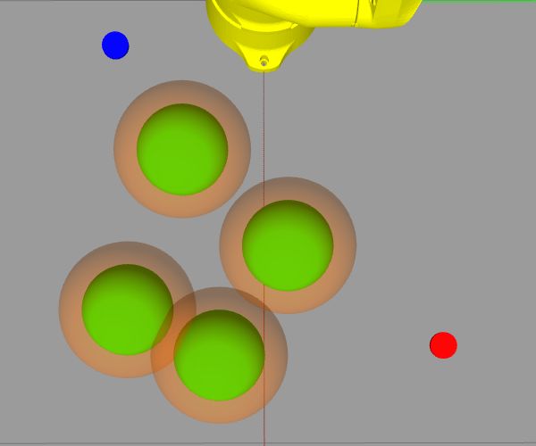
Robotics 2023, 12, 7                                                                                             5 of 24

                                            e
                       end-effector pose Hw,des  . For the manipulator, which is shown exemplarily in Figure 1, the
                       first m joints qm ∈ Rm are assigned to the red framed anthropomorphic arm (I) and the last
                       o joints qo ∈ Ro belong to the blue framed spherical wrist (II). We considered 3 ≤ m < n
                       and 3 ≤ o < n so that the n = m + o robot DOFs are partitioned in such a way that any pose
                       can be achieved in the reachable workspace. To this end, the robotic model is decomposed
                       into the qm associated part for translational displacement and the qo relating system for
                       rotational alignment to reduce the number of variables in the equations describing both
                       associated models, respectively [21,71]. Thus, instead of evaluating the entire kinematic
                       chain, two reduced chains are considered. The connection of the two systems is defined
                       at the wrist frame {ς}, where the so-called wrist point pw = [ pw,x , pw,y , pw,z ]T ∈ R3 is
                                                                                      ς      ς   ς   ς

                       located. The wrist point can be obtained by equating the traversed kinematic chains that
                       converge in {ς} starting in the {w} and the {e} frame, respectively. Starting at {e}, the
                       desired end-effector pose can be projected onto the flange by
                                                     "         #
                                                         f   f
                                               f       Rw pw        e
                                                                                −1            f
                                              Hw =      T
                                                                 = Hw,des H ef          e
                                                                                    = Hw,des He                  (1)
                                                       0    1

                       using the tool-specific transformation matrix H ef .
                                                                                           f
                            The orientation of the z f -axis of the flange is denoted by r w,z and can be obtained from
                                              f
                       the third column of Rw . The wrist point
                                                                  f         f
                                                          pςw = pw − d f r w,z ∈ R3                                 (2)

                       can be calculated based on (1) and the length d f of the last link ending at the flange.
                                                                                                          ς
                       Using (2) as the left-hand side and the position vector of the direct kinematics Hw (qm ) as
                       the right-hand side, a system of equations can be set up to determine qm . When considering
                       a redundant robot with m > 3 and n > 6, additional constraints to the nullspace must be
                       introduced to solve the system uniquely [72]. Apart from the possible nullspace, there are
                       generally up to four valid solutions describing the shoulder left or right and elbow up or
                       down configurations [73]. The so-called rotation correction can be determined by
                                                           f        T   f          f
                                                         Rm = ( Rm         w
                                                                 w ) Rw = Rm Rw .                                   (3)

                                                                                                                      f
                       Via the ZYZ-sequence [74], which is based on the joint structure of the spherical wrist, Rm
                       can be implied for the joints qo . This in turn yields ambiguous solutions known as wrist
                       top and wrist bottom [73], respectively. This doubles the maximum number of possible
                       configurations mentioned above, so that up to eight solutions can exist for one desired pose
                         e
                       Hw,des . In this contribution, an automatic selection was introduced, which performs an
                       evaluation of the most-suitable joint configuration and selects it for the movement. Jumps
                       between the up to eight solutions are avoided, and the common boundaries are considered.

                       2.2. Decomposition of Differential Kinematics
                            Based on the method presented before, the robot model is decomposed for the follow-
                       ing control architecture. The separation into a translational and a rotational part allows
                       the consideration of external boundary conditions, e.g., for the avoidance of obstacles,
                       to be directly assigned to specific joints in the robot’s kinematic chain. Thus, the DOFs
                       considered in the optimization-based control approach are reduced by kinematic analysis,
                       reducing the computational costs. Differential kinematics rather than direct kinematics
                       was taken into account to avoid algebraic loops in the online computations [75] and for a
                       more straightforward restriction of the nullspace in the case of redundant robots [57,69].
Robotics 2023, 12, 7                                                                                              6 of 24

                       The transformation of joint velocities q̇ ∈ Rn into Cartesian velocities can be performed by
                       differential kinematics using

                                                                    ṗew

                                                                           = Jwe (q) q̇ ∈ R6 .                       (4)
                                                                    ωew

                       The translational velocity of the end-effector with respect to the {w} system is described by
                       ṗew ∈ R3 , while ωew ∈ R3 expresses the corresponding angular velocities [69]. The nonlinear
                       geometric Jacobian matrix:

                                                               Jtrans     J             Jtrans,2
                                               Jwe (q) =               = trans,1                   ∈ R6×n            (5)
                                                                Jrot        Jrot,1       Jrot,2

                       is introduced. From (5), it can be seen that the entire Jacobian consists of a translational
                       and a rotational part. Transferring the approach of Section 2.1 to the decomposition of the
                       manipulator, Jtrans,1 and Jrot,2 represent the associated terms in the differential kinematics,
                       and the submatrices Jtrans,2 and Jrot,1 denote cross-couplings, respectively. Instead of using
                       the entire transformation from (4), the differential kinematics is split as well. Based on the
                       decomposition analyzed in the inverse kinematics, translation is performed by the first m
                       and orientation by the last o robot joints [57]. According to the general matrix computation
                                                                                      f
                       as described in [69], the matrices Jw,trans (qm ) ∈ R3×m and Jm,rot (qo ) ∈ R3×o are introduced
                                                            ς

                       and used subsequently instead of (5). The DOFs due to the cross-couplings are eliminated
                       as a consequence in the transformation performed in (4) for the full robot system. This
                       means that the joints qm no longer have an active influence on the end-effector’s orientation
                       and qo cannot be used for the translational positioning of the {e} frame. Further, two
                       controllers for qm and qo were designed separately and then coupled.
                                                                                ς
                             One controller controls the positioning using Jw,trans (qm ), and the other controller
                                                      f
                       adjusts the alignment with Jm,rot (qo ). Analogous to the evaluation of inverse kinematics in
                       Section 2.1, there is no loss of DOFs in the Cartesian space, and due to controller couplings,
                       the entire workspace is still reachable.
                                                                                   ς
                             It should be emphasized that the translational part Jw,trans (qm ) refers to the wrist point
                         ς
                       pw , while the orientation of the {ς} system is irrelevant in this context. Using (1) and (2),
                       the desired wrist point is obtained from pew,des , and an orientation error follows from the
                                                                                                        f
                       wrist positioning using the first m robot joints. In turn, the Jacobian Jm,rot (qo ) for the
                       rotational part refers to the {m} system localized in the robot’s elbow, the last joint of the
                       anthropomorphic arm, as shown in Figure 1. The link between the {m} and the {ς} system
                       exhibits a constant length and is aligned along the rotation axis of the first spherical wrist
                       joint. Thus, this DOF only changes the alignment and not the displacement between both
                       systems, and the two kinematic chains can be connected in this way.

                       3. Optimal Trajectory Control Using Decomposed Differential Kinematics
                            To implement fast online control, Section 3.1 presents a computationally effective
                       planning scheme involving all robot joints to generate an initial trajectory that does not take
                       external disturbances into account. It can be used when the workspace is not constrained
                       and serves as a reference in a warm start of the following optimization. An automatic
                       selection is introduced that identifies the most-suitable joint configuration for the desired
                       terminal pose. The up to eight possible solutions of the inverse kinematics are checked
                       for jumps for the planned pose transition, and the solution with the largest distance
                       to the joint boundaries is selected. In Section 3.2, the constrained OCP is formulated,
                       with the translational part of the decomposed system from Section 2.2 as the underlying
                       model. The OCP is evaluated on a receding time horizon, i.e., controlling the robot using
                       NMPC. Meanwhile, the orientation of the end-effector is considered separately using the
                       controller presented in Section 3.3. In Table 1, the main difficulties and characteristics of
                       the two controllers are listed as an overview. Special attention has to be paid to the wrist
                       position, which is iteratively placed by the NMPC and determines the starting pose for the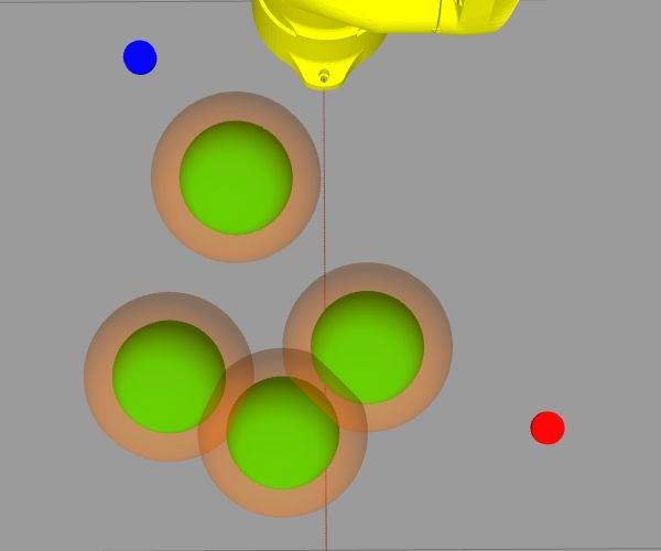
Robotics 2023, 12, 7                                                                                                   7 of 24

                       orientation controller. The combination of the two controllers provides the overall control
                       of the robot, and both are calculated subsequently in each iteration. If the orientation
                       controller, based on the Jacobian transpose controller here, is also implemented as a second
                       NMPC, the controllers would have to be evaluated sequentially and, therefore, would
                       be time consuming because of the dependency with respect to the reference pose at the
                       {m} frame.

                       Table 1. Comparison of the difficulties and characteristics of the decomposed robot model illustrated
                       in Figure 1 for optimal trajectory control achieving low computation times in online calculations.

                              Properties           I: Anthropomorphic arm               II: Spherical Wrist
                               intended           • translational movement              • orientation control
                                  use             • avoiding obstacles in               • alignment for
                                                    disturbed environment                 desired rotation
                              constraints         • iterative solving                   • depending on
                                                    starting at fixed base                wrist movement
                                                  • environmental, state                • standard controller
                                                    and input constraints                 bounded to limits
                                                  • consideration of the                • compensation of
                                                    distance between                      rotation correction
                                                      ς
                                                    pw and end-effector
                                control           • control of qm using                 • control of qo with
                                                    NMPC                                  Jacobian controller
                                                  • optimization with                   • reaction based on
                                                    known reference                       wrist displacement
                                                                                          (from NMPC)
                              singularity         • configuration bounded               • Jacobian transpose
                              avoidance             to objective function                 using no inversion
                                                    with regularization                   in calculations
                                                  • preselection of the                 • unit quaternions pre-
                                                    closest solution                      venting a Gimbal
                                                                                          lock [74]

                       Remark 1. Here, only a multi-DOF robot with an anthropomorphic structure and revolute joints
                       is discussed, so that an independent assignment of the joints to a translational and rotational motion
                       in the Cartesian space can be performed. This design as an open or closed kinematic chain is the
                       most common setup of standard industrial robots. A transfer of the approach to other manipulator
                       types can be applied if the robotic model admits a decomposition according to the specification.

                       3.1. Polynomial Trajectory Planning
                            An initial planning for all n robot joints is performed before the online controlled robot
                       movements start. To generate a reference trajectory, a polynomial approach in the joint
                       space is utilized to connect the initial end-effector pose represented by the homogeneous
                       transformation Hwe (q(t0 )) at time t0 ∈ R≥0 with the desired terminal pose Hw,dese     at time
                       t1 = t0 + T, obtaining a continuously differentiable trajectory. The transition time T ∈ R>0
                       must be chosen so that the dynamic joint limits of the robot are not violated. To check
                                    e
                       whether Hw,des   is an admissible pose with the mounted end-effector according to the given
                       bounds in the robot’s data sheet, (2) can be used to validate the wrist point. As mentioned
                       in Section 2.1, up to eight possible joint configurations can be determined for the given
                       pose at t1 . From the set of possible solutions of the inverse kinematics, the configurations
                       that are not included in the reachable joint space:

                                                      Q := {q ∈ Rn | qmin ≤ q ≤ qmax }                                    (6)
Robotics 2023, 12, 7                                                                                                                        8 of 24

                       are excluded. To connect the initial joint setup q(t0 ) and the remaining β ≤ 8 terminal
                       configurations Q β (t1 ) = [q1 (t1 ), . . . , q β (t1 )] ∈ Rn× β , the polynomial:

                                                                                     7
                                                                           γ(t) =   ∑ λ j t j ∈ Rn                                             (7)
                                                                                    j =0

                       is introduced. The eight unknowns λ j , j ∈ {0, . . . , 7} for each of the n joints can be
                       determined, respectively, from the eight boundary conditions:

                                      ( j)                          ( j)            ( j)
                                    γ i ( t0 ) = q ( j ) ( t0 ),   γ i ( t1 ) = q i ( t1 ),   j ∈ {0, . . . , 3}, i ∈ {1, . . . , β}           (8)

                                                                                    (0)
                       for each configuration i. In (8), γi (t) = γi (t) applies, and the derivatives are given by
                        ( j)
                       γi (t), which describe the associated velocity, acceleration, and jerk, respectively. The
                       velocity bounds can be measured or formed by the inverse evaluation of (4). Without loss
                       of generality, the acceleration and jerk are chosen to be zero at the beginning and at the end
                       of the transition. The acceleration bounds can alternatively be transformed by introducing
                       the time derivative of the Jacobian in (5) [69]. In order to drop the solutions that contain an
                       unnecessary change at the shoulder, elbow, or wrist of the robot, all β transitions connecting
                       q(t0 ) with the configurations in Q β (t1 ) are sampled by tγ ∈ R>0 and examined for jumps.
                       From the remaining r ≤ β possibilities that do not involve jumps, the configurations that
                       are furthest away from the joint boundaries with the corresponding joints are selected from
                                  n                                            o
                               max min qi,ρ (tγ ) − qi,min , qi,max − qi,ρ (tγ ) ,               ρ ∈ {1, . . . , r }, i ∈ {1, . . . , n}.      (9)
                                ρ            i

                             Each joint i is evaluated individually at each sample step tγ . If several joint configu-
                       rations exhibit the same distances to the bounds, the maximum operator in (9) is used to
                       select the configuration that maintains the greatest distance from the boundaries qmin and
                       qmax , considering all sampling steps tγ . If the coupling of the two checks were reversed, a
                       joint that is far from its bound could compensate a joint close to its respective bound in the
                       evaluation. Since the planning is implemented in the joint space, no consideration of the
                       Euler angles [74] in Cartesian space is necessary, which prevents representation singularities.
                       Using the introduced procedure in (9), an automatic selection method of the most appro-
                       priate kinematic configuration is introduced, eliminating the need for a manual selection,
                       required by most of the inverse kinematics tools [63,65,67,68].

                       3.2. Optimization-Based Translational Trajectory Control
                            For the translational motion in the robot’s workspace considering obstacles, a con-
                       strained optimization problem with a fixed end time τ1 = τ0 + N ∈ R>0 is introduced.
                       The prediction horizon of the OCP is defined by N ∈ R>0 and is starting at τ0 = tδ .
                       Thereby, tδ ∈ R≥0 describes the current sampling step. With the underlying model of the
                       decomposed differential kinematics from Section 2.2, the joint velocities:

                                                        U := {u ∈ Rm | − q̇m,max ≤ u(τ ) ≤ q̇m,max }                                        (10a)

                       are chosen as fictitious inputs of the OCP. As can be seen from (10a), only the first m joints of
                                                                                                  ς
                       the robot are taken into account for the displacement of the wrist point pw . The end-effector
                       orientation is adjusted subsequently by means of qo . Standard industrial robots are usually
                       controlled using joint position controllers [63,65] so that the joint angles qm to command
                       the translational motion of the robot can be obtained by solving q̇m = u. Furthermore,
                       the OCP:                                 Z τ
                                                                   1
                                                   min F (u) =       l u, pςw (qm ), q̈m , µ dτ                   (10b)
                                                            u∈U                τ0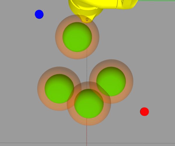
Robotics 2023, 12, 7                                                                                                        9 of 24

                       is considered by minimizing the running cost:
                                                                                                  T ς
                        l u, pςw (qm ), q̈m , µ = µu uT u + µq̈ q̈Tm q̈m + µ p pw,des − pςw (qm )
                                                                               ς
                                                                                                     pw,des − pςw (qm ) (10c)

                       over the time interval τ ∈ [τ0 , τ1 ]. The elements from µ = [µu , µq̈ , µ p ]T ∈ R3 can be used
                                                                                                  ς
                       to weight the individual terms in (10c). The desired wrist position pw,des is derived from
                       the desired end-effector pose using (2). If a reference trajectory is specified, e.g., with the
                       procedure introduced in Section 3.1, using MoveIt for task-level motion planning [76] or
                       based on the techniques summarized in [14], the Lagrange function shown in (10c) aims for
                       trajectory tracking. Alternatively, only the terminal position could be passed to (10c) as a
                       reference, which is called a local motion planning problem [35]. By considering the input u
                       in (10c), the agility can be influenced, and the relating part also represents a regularization
                       term, to prevent singular arcs [43]. In order to further prevent singularities, it is possible
                       to include the manipulability measure into the running cost as well [77]. In practice, the
                       integral listed in (10b) is discretized by a sum over k ∈ N>0 temporal grid points for the
                       numerical implementation. Enabling an influence on the rate change, q̈m is also included
                                                                    ...
                       in (10c). The acceleration q̈m and the jerk q m result from the discrete differentiation of the
                       input u, respectively. Based on the system formulation:
                                           ς                                                                 ς
                                      d pςw                                                           ς

                                              J      (q ) u                                          pw (τ0 )    p
                                            = w,trans m       , τ > τ0                    with                 = w,0 ,      (10d)
                                      dτ qm         u                                                qm (τ0 )    qm,0
                                                                                      ς
                       the variables in (10b) can be determined. Here, pw,0 describes the initial wrist position and
                       qm,0 the initial joint angles at time τ0 . Using the inequality constraints:

                                                         qm,min ≤ qm ≤ qm,max
                                                          ( j)         ( j)    ( j)
                                                                                                                            (10e)
                                                     −qm,max ≤ qm ≤ qm,max ,                j ∈ {2, 3},

                       the system (10d) is constrained to the reachable joint space, since the selected joint angles qm
                       must be inside the valid bounds of (6). Applying the constraints in (10e) to the acceleration
                                    ...
                       q̈m and jerk q m , non-adjustable changes can be avoided. The respective bounds are usually
                       known for standard industrial robots and can be taken from the appropriate data sheet,
                       e.g., given by [63].
                             Obstacles are subsequently modeled as spheres to illustrate the approach [78], but can
                       also be described by using sophisticated techniques as, e.g., by the evaluation of tetrahedral
                       meshes or polyhedra [21,79,80]. Let ν denote the number of obstacles in the Cartesian space.
                       These are assumed moveable and centered at pνw,i (τ ) ∈ R3 , i ∈ {1, . . . , ν}, imposing the
                       inequality constraints:
                                                     q
                                        ri + d f +       ( ae )2 + (de )2 < | pςw − pνw,i (τ )|,       ∀i = 1, . . . , ν.   (10f)

                       Due to the decomposition of the robot model, the resulting orientation of the end-effector
                       during motion is not known in the optimization. Therefore, the length of the spherical
                       wrist plus the DH parameters ae ∈ R and de ∈ R of the end-effector are also defined as
                       a sphere around the wrist point. This is added to the radius ri ∈ R>0 of each obstacle to
                       obtain a safe distance.
                            For example, to perform horizontal motion only or to prevent touching the ground,
                       the height:
                                                       ς          ς       ς
                                                     pw,z,min ≤ pw,z ≤ pw,z,max                             (10g)
                       of the robot’s workspace can also be optionally bounded. Constraining of the OCP (10)
                       by adding (10g) usually increases the computational times significantly, which will be
                       demonstrated in Section 4.1. However, by reducing the robot model in (10d), it is possible
                       to include further constraints influencing the robot’s behavior.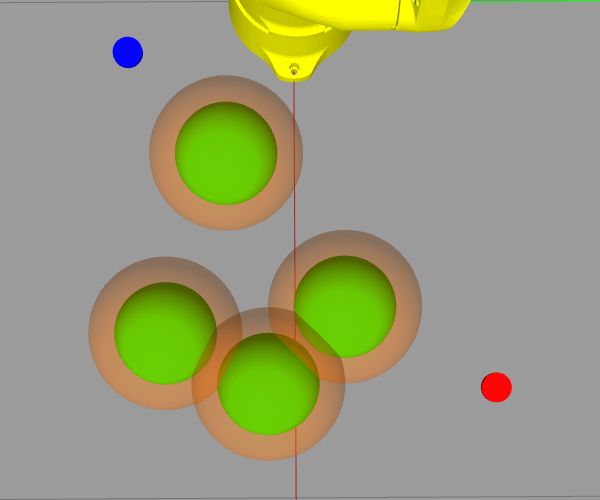
Robotics 2023, 12, 7 10 of 24
NMPC can be applied by solving the presented OCP on a receding horizon with a
suitable prediction length N. Both the initial wrist position and the joint angles can be
obtained from the measured joint angles of the robot. Direct multiple shooting is used for
the numerical evaluations, which considers an initial value problem in each time interval
[τκ −1 , τκ ], κ ∈ {1, . . . , k} [81]. Hence, k initial value problems have to be solved in total.
Since the subintervals can be solved independently, parallelization can be used. To ensure
a continuous transition between intervals, boundary conditions must be imposed so that
the boundary values of the adjacent intervals are identical [82]. For a warm start, the initial
estimates of the optimization variables and the input can be set for each step τκ by the
procedure presented in Section 3.1. According to [81], an approach is used here that first
discretizes and then optimizes, converging to local or global minima depending on the
solver settings and the weightings chosen in the quadratic objective function (10b).
3.3. Jacobian Transpose Controller Achieving Desired Orientation
To achieve the desired orientation, a controller is presented to track the last joints qo of
the robot’s kinematic chain accordingly. For this purpose, the Jacobian transpose controller
is used and applied to the problem formulation [57]. This implies less computational effort
compared to the Jacobian inverse controller commonly used in robotics and can be utilized
to cross kinematic singularities [69]. When solving the NMPC formulated in Section 3.2,
a joint configuration qm (tδ ) for the first m robot joints of the kinematic chain is obtained
for each iteration step. These define the orientation of the {m} frame at the robot’s elbow,
which results in the rotation matrix Rm w ( qm ). This matrix can be used in (3) to determine the
f
deviation matrix Rm (qm ) between the desired end-effector orientation, transformed to the
flange { f } and the current wrist orientation governed by qm . Therefore, the corresponding
f f
unit quaternions [ηm (qm ), (ζ m (qm ))T ]T can be derived [83,84]. They specify the desired
unit quaternions with respect to the {m} frame depending on the displacement of the
{ς} system at the wrist point performed by the NMPC. From the joint angles qo (tδ ) at
f f
sampling step tδ , the current [ηm (qo ), (ζ m (qo ))T ]T unit quaternions can be calculated. The
orientation error:
f f f f f f f
ẽm = ηm (qo ) ζ m (qm ) − ηm (qm ) ζ m (qo ) − S ζ m (qm ) ζ m (qo ) ∈ R3 (11)
between these unit quaternions can be inferred, where the skew symmetric operator [85] reads
0 − s3 s2
S ( s1 , s2 , s3 ) = s3 0 − s 1 ∈ R3 × 3 . (12)
− s2 s1 0
It should be emphasized that η = 1 holds true for the real part of the unit quaternions
when the orientation is aligned, and thus, the orientation error in (11) can be expressed as a
3D quantity [86]. Using
f T f
q̇o = Jm,rot K ẽm , (13)
the feedback is imposed, including the positive definite matrix K ∈ Ro×3 and the Jacobian
determined in Section 2.2. The weighting matrix K is bounded to the sample time and
influences the speed of convergence. The required joint angles qo to control the robot
are obtained by the integration of (13). In order to analyze the stability of the orientation
controller, the Lyapunov function:
f f 2 f f T f f
V = ηm ( q m ) − ηm ( q o ) + ζ m (qm ) − ζ m (qo ) ζ m (qm ) − ζ m (qo ) (14a)
is considered. After substituting the propagation equations for quaternions [86] into the
rate of change:
f T f
V̇ = − ẽm K ẽm (14b)Robotics 2023, 12, 7 11 of 24
of (14a), the asymptotic stability of the orientation controller can be concluded. Thus, the
controller converges to the desired orientation and is able to cross singularities, whereas, in
contrast to the Jacobian inverse, it may deviate during the transition phase [58,69].
4. Simulation Results and Evaluation
To show that standard computer hardware is sufficient for the online calculations of
the introduced NMPC for the translational motion including Cartesian and joint constraints
coupled with the Jacobian transpose controller for the orientation correction, a standard
computer with 16GB RAM and an Intel Core i7-8550U processor running Linux Ubuntu
18.04 was utilized. The iterative solution of the OCP is calculated using the MATLAB-
interface [87] from C AS AD I [88] with the interior-point (IPOPT) algorithm [89]. As can be
seen in Figure 2, the standard industrial 6-DOF robot Stäubli TX2-90 with a black rod as
the end-effector and the DH parameters from Table 2 was used to present the introduced
approach. Based on the decomposition performed in Section 2.2, both controllers consider
different kinematic chains, respectively. Thus, the associated DH parameters to the {m}
ς
system and the wrist point pw are also listed in the table. The n = 6 revolute joints are
equally partitioned with m = 3 and o = 3 for the translational and rotational controllers.
Table 2. Denavit–Hartenberg (DH) parameters of the considered 6-DOF industrial Stäubli TX2-90
manipulator.
i ai (mm) αi (rad) di (mm) θi (rad)
w 0 0 −478 0
1 50 −π/2 478 q1
2 425 0 0 q2 − π/2
3/m 0 π/2 50 q3 + π/2
ς 425 0 50 q3
4 0 −π/2 425 q4
5 0 π/2 0 q5
f 0 0 100 q6
e 0 0 150 0
elbow shoulder
{m} zw
ym {w} yw
xm
zm xw
z0 y
0
{0}
wrist x0 Iν
ς
pw
ye xe
{e} ze
Figure 2. Standard industrial 6-DOF manipulator Stäubli TX2-90 [63] with an end-effector, visualized
in G AZEBO [64,90]. The exemplary movement starts at the blue marker and ends at the red one. The
green obstacles are only considered in Sections 4.3 and 4.4, but are not present in Section 4.2.
The evaluation consisted of four different demonstrations to highlight the perfor-
mance of the NMPC approach based on the decomposed robot model. In Section 4.1, theRobotics 2023, 12, 7 12 of 24
computation times of the introduced approach are evaluated and compared to an NMPC
considering the full robot system. This highlights the significant difference in the computa-
tional costs between those approaches. Despite the decomposition of the model and the
controller couplings, no losses in the applicability by the approach occur, which is shown in
the following three evaluations. The trajectory tracking accuracy in the undisturbed case is
discussed in Section 4.2 to show that the method can be used as an online motion controller.
Subsequently, in Section 4.3, obstacles are placed in the environment. In the presented
scenario, the end-effector must be guided between them without causing collisions. The
obstacles are not taken into account for the trajectory planning described in Section 3.1, but
will be avoided by the online controller introduced in Section 3.2, which perceives them
only within its predictive horizon. Finally, in Section 4.4, moving obstacles are considered
and the collision-free guidance of the end-effector in this setup is investigated.
4.1. Quantitative Analysis of the Computation Times
In the analysis of the reduction in the computation times, the presented approach was
compared to an NMPC that considers the full robotic model. Using the Stäubli TX2-90,
the NMPC based on the full system utilizes n = 6 joints as decision variables in each
optimization step and incorporates both translation and orientation by Jwe (q) from (5). On
the contrary, the decomposed system requires only m = 3 decision variables in its OCP
and controls the orientation in parallel with the remaining three DOFs using the coupled
Jacobian transpose controller. It should be emphasized that (10c) must be extended in the
NMPC of the full system to include orientation as well. The objective functions of the two
systems differ, but each was designed for the quantitative comparison. As listed in Table 3,
three different scenarios consisting of no obstacle, one obstacle, and one obstacle including
height constraints were compared to analyze the computation times. Additionally, two
different prediction horizons N1 = 100 ms and N2 = 200 ms partitioned with k1 = 10 and
k2 = 20 grid points were considered, achieving discrete intervals with a length of 10 ms,
respectively. The discretization of the inputs to be determined corresponds to the update
rate of the robot controller. Various converging point-to-point (PTP) movements covering
the entire workspace of the robot were run multiple times, and the average computation
time t̄ per optimization step was recorded. This time and the standard deviation σ, which
expresses the fluctuation of t̄ required for one OCP, denotes the online capability of the
NMPC. Note that the optimization was carried out until an optimal solution was found,
but could be further shortened by limiting the maximum iterations, as done in [91]. Here,
the stop condition for the objective function (10b) was set to a tolerance of 10−8 , and if
below this limit, the value did not change more than 10−6 , indicating a minimum.
Table 3. Comparison of the averaged computation times t̄ with the standard deviation σ per opti-
mization step of the respective NMPC.
Point-to-Point Decomp. System Full System
Movement t̄ ± σ (ms) t̄ ± σ (ms)
N1 26 ± 1 130 ± 12
without obstacles
N2 30 ± 2 216 ± 21
N1 27 ± 2 153 ± 53
with obstacle
N2 33 ± 2 209 ± 9
with obstacle N1 29 ± 2 230 ± 136
and height constraints N2 36 ± 6 284 ± 112
From Table 3, the comparison between the decomposed and the full system shows
that the decomposed system requires only 10 % to 20 % of t̄ to achieve an optimal solution
and possesses lower deviations σ, independent of the scenario or the prediction horizon.
Both t̄ and σ are important factors to be considered using NMPC in varying environments.Robotics 2023, 12, 7 13 of 24
The Jacobian transpose controller evaluates the orientation error in each iteration and is
only constrained to the gain matrix K.
It can be seen that the average computation times t̄ for the full system increased signif-
icantly with the complexity of the scenario. This effect did not occur with the decomposed
model, as the full system involves more nonlinearities, which must be taken into account
to solve the OCP. On the one hand, higher computational costs yield lower possible update
rates of the NMPC, which restricts the ability to act in rapidly varying environments. On
the other hand, it is evident from Table 3 that N2 increased the computation times for the
full system by up to 67 %, in contrast to t̄, when N1 was chosen. This means that the choice
of the prediction horizon limits the online capabilities. Using the decomposed robot model
approach, the evaluation times increased by a maximum of 24 % using N2 instead of N1 .
Thus, the comparison of both the absolute and the relative computation times revealed a
significantly higher performance of the presented decomposition-based method.
A second important factor is σ, which is a measure of the reliability to achieve t̄.
Smaller standard deviations, even between different scenarios, indicate that t̄ is more likely
to be achieved. In contrast to the NMPC considering the full system, the lower σ of the
decomposed system also allows for easier applicability to different tasks, since the NMPC
does not converge for an unexpectedly long time in a more complex scenario. The choice of
the control horizon is determined by the length of expected calculation times and should be
kept as short as possible. Referring to Table 3, the control horizon can be set more reliably
using the decomposed approach. The NMPC controller remains capable in online operation
without delaying the robot’s motion, resulting in t̄ being larger than the set control horizon
in the implementation.
4.2. Trajectory Tracking Accuracy of the Controller
In Section 4.1, the significant reduction of the computational costs is presented. Fur-
thermore, it is shown that this did not lead to any restrictions in the motion behavior of the
robot. The simulative setup for evaluating the introduced approach involving the NMPC
and the orientation controller was built in G AZEBO [64]. The joint position controlled robot
shown in Figure 2 is commanded by means of ROS [65,90]. The prediction horizon was
chosen as N = 100 ms with k = 10 grid points per iteration, while the control horizon
involved four discretization steps of 10 ms each. This means that, for all four consecu-
tive updates of the robot commands, the solution from the buffer was used before being
updated. Considering the average computation times from the previous subsection, this
allows for online calculations without delaying the robot’s motion due to the too long
computations solving the OCP. Finally, the gain matrix for the orientation control was set
to K = diag(20, 20, 20), and the weights of the NMPC’s running costs in (10c) were chosen
to be µ = [104 , 102 , 104 ]T .
We omit the comparison with the full system in the following evaluations, on the
one hand, for the sake of readability and, on the other hand, to avoid having an unfair
comparison realized. As shown in Section 4.1, no delay-free execution can be realized for
the chosen N using the full system, which distorts the comparison. Depending on the
controller settings, we observed only minor to no deviations between the results in internal
comparisons, depending on the scenario.
As shown in Figure 2, the end-effector has to move from the blue marker with
pew,0 = [110, −350, −405]T mm at t0 to the red marker with pew,des = [780, 390, −405]T mm
at t1 . None of the green obstacles are considered in this subsection when performing the
trajectory tracking analysis, and they are only drawn in preparation for the next scenario.
The desired orientation was set to Rew,des = diag(−1, 1, −1), meaning that the end-effector
has to point vertically downwards. However, all other orientations reachable in the ma-
nipulator’s workspace can also be realized. As explained in Section 3.3, the Jacobian
transpose controller is asymptotically stable and does not induce singularities in individual
joint configurations, e.g., compared to the Jacobian inverse controller. As illustrated in
Figure 3b with dashed lines, the set point change of the desired position using the polyno-Robotics 2023, 12, 7 14 of 24
mial approach from Section 3.1 starts at t0 = 0.5 s and ends at t1 = 2 s. The demonstration
scenario involving a short transition time T = 1.5 s and a long path is representative for
movements between all reachable poses in the workspace of the manipulator. If T is not set,
e
the desired terminal pose Hw,des , will be approached by minimizing the objective function
within the NMPC, just bounded to the given OCP constraints.
500
pew [mm]
x xdes
0 y ydes
z zdes
−500
0 t0 1 t1 3 4
(a)
30 x
p̃ew [mm]
y
0 z
−30 k·k
0 t0 1 t1 3 4
(b)
0.06 ζ1
ζ2
ẽm
f
0.03
ζ3
0
0 t0 1 t1 3 t [s]
(c)
Figure 3. Trajectory of the end-effector starting at t0 = 0.5 s and ending at t1 = 2 s in an undisturbed
environment for tracking accuracy analysis in 3D space. (a) Trajectory tracking of the pre-planned
trajectory marked by the subscript “des”, which is planned in the joint space and transformed
into the Cartesian space. (b) Absolute displacement of the end-effector p̃ew = pew,des − pew to the
reference trajectory and the individual translational parts depending on the length de = 150 mm of
the end-effector. (c) Orientation error (11) in quaternion representation.
The pre-planned trajectory is generated by using the polynomial depicted in (7) in the
joint space. The computation time of approximately 1 ms required for this involving the
automatic joint configuration selection ensures an almost instantaneous start. Subsequently,
this is transformed to the Cartesian space. As can be seen in Figure 3a, the reference
trajectory exhibits rounded deviations, for example at t = 1.2 s in pew,z,des , compared to
a trajectory that would be directly planned in the Cartesian space, because the joints are
actuated uniformly over T here. In turn, the evaluation of the orientation by, e.g., roll-pitch-
yaw [74] is omitted by using the joint space, which could be singular in the representation.
In the evaluation of the end-effector’s translational deviation, both controllers must
be taken into account. It should be noted that the end-effector position is composed of the
positioning of the wrist point by the NMPC and the alignment by the orientation controller.
Both a too slow control of the wrist point and an incorrect orientation of the end-effector
would lead to a deviation from the end-effector’s reference trajectory. In Figure 3b, the
individual error components of p̃ew = pew,des − pew and the absolute distance k p̃ew k to the
reference trajectory at each time step are shown. Despite the short transition time T and
the long displacement along the trajectory, resulting in a rapid change of poses, only small
deviations can be detected. Compared to a common path tracking task, it must be taken
into account that, in the analysis of the trajectory tracking accuracy, a slight lag also leadsRobotics 2023, 12, 7 15 of 24
to notable deviations. As can be seen in Figure 3b, especially the errors of pew,x and pew,y
exhibit small deviations, which converge to zero in the end, so that no stationary error
remains. The small lag in the xw yw -plane during the motion results from the parameterized
smoothness of the orientation controller, since it must perform the rotation correction in
each iteration step due to its constantly shifting reference {m} system. The NMPC places
ς
the wrist point pw very accurately so that the reference system of the upper kinematic chain,
used for the orientation control, is moved further and further by the NMPC. Therefore,
a permanent adaptation in (11) governed by K is necessary. The rotation error is shown
in Figure 3c, where each of the imaginary unit quaternion error components can take a
maximum value of one. Thus, it can be seen that the orientation error was very small in
this case. Even though, the end-effector is chosen to be relatively long with de = 150 mm.
As a result, a larger deviation was enforced for a better illustration here. If de is chosen
shorter, the amplitudes in Figure 3b decrease. In total, just small deviations from the
pre-planned trajectory and, thus, accurate trajectory tracking can be observed when using
the presented approach.
4.3. Trajectory Control in Disturbed Environment With Fixed Obstacles
In the evaluation involving obstacles, the same control setup as in Section 4.2 was
utilized, but as illustrated in Figure 2, the scenario now included ν = 4 obstacles and
pew,0 = [110, −350, −445]T mm and pew,des = [780, 390, −445]T mm were set 40 mm lower
in the zw -direction. This small lowering of the reference trajectory would cause ground
contact, which should be prevented by the controller. Starting from the blue marker in
Figure 4, the first obstacle was placed close to the reference trajectory so that the boundary
condition (10f) had to consider the mentioned safety distance, since the NMPC has no
knowledge about the orientation controller, which adjusts the desired orientation. In the
extreme case, when the end-effector would be vertical, the NMPC should directly leave
the reference trajectory to avoid collisions. As shown in Figure 4, the two consecutive
obstacles on the left-hand side are crossed by the blue reference and disturb the tracking of
the pre-planned trajectory in xw yw -plane. Additionally, the central obstacle (Iν ) presents
a difficulty in conjunction with the height constraint (10g), since the NMPC must deviate
significantly from the reference and take a remarkable detour to reach Hw,des e . The NMPC
only considers the obstacles within the prediction horizon and has no information about
them before. In the accompanying video [92], the orientation error and the wrist point
tracking are also shown, in addition to the executed robot movements. For the sake of
readability, the evaluation is omitted in this section and reference is made to Section 4.2.
Iν
Figure 4. Resulting trajectories of the end-effector pew (t) governed by the NMPC and orientation
controller in the scenario from Figure 2. The motion starts at the blue marker and ends at the red
marker. The reference trajectory (blue) according to (7) crosses the obstacles (green). Without a height
ς
constraint for pw,z , the motion results in an upward swerve (yellow). Activating (10g), the spheres
are avoided in the xw yw -plane (red).
From Figure 5a, the trajectory of the end-effector can be taken in the case where the
ς ς
wrist point pw is only constrained by pw,z,min = −228 mm in (10g) involving no upperRobotics 2023, 12, 7 16 of 24
height limit, so that the ground will not be touched. A deviation from the dashed reference
trajectory due to the obstacle avoidance can be seen. Especially with respect to pew,x and
pew,y , it is obvious that the trajectory controller tries to follow the reference trajectory under
consideration of the given constraints, but a delay is recognizable. From Figure 4, it
becomes even clearer that the yellow trajectory in the xw yw -plane follows the arc of the
blue reference quiet accurately. The obstacles are avoided by swerving in the zw -direction,
which is confirmed by the green line in Figure 5a. Due to the chosen IPOPT algorithm and
depending on the length of the control horizon, which has to be chosen according to the
computation times of the controller’s online calculations, small repeated repulsions of the
end-effector can be detected in Figure 4 while avoiding the obstacles tightly.
500
pew [mm]
x
0 y
z
−500
0 t0 1 t1 3 4
(a)
500
pew [mm]
xdes
0 ydes
zdes
−500
0 t0 1 t1 3 t [s]
(b)
Figure 5. Trajectory tracking of the blue curve in Figure 4 starting at t0 = 0.5 s and ending at t1 = 2 s
in a disturbed environment involving ν = 4 fixed obstacles. (a) No upper height limitation of
the Cartesian space. Analogous to the yellow trajectory in Figure 4, the manipulator moves over
ς
the obstacles. (b) Constraining the height by −228 mm ≤ pw,z ≤ −145 mm in (10g) for obstacle
avoidance in the xw yw -plane, as the red curve in Figure 4.
By reducing the computational costs, short evaluation times of the NMPC can be
achieved, even if additional constraints are inserted, which further influence the robot’s
behavior. This means that, by decomposing the differential kinematics, not only an accurate
controller can be designed, but also, it can be used more flexibly. In order to demonstrate
this, the maximum height in the Cartesian space was constrained in the further analysis.
ς
The height constraint −228 mm ≤ pw,z ≤ −145 mm of the wrist’s workspace forces the
controller to avoid the obstacles by a planar motion. The lifting of the end-effector is thus
e
suppressed. Therefore, Hw,des can just be approached by a significant deviation from the
reference trajectory, mainly disturbed by the central obstacle (Iν ). A noticeable change in
the movement compared to the dashed lines can be noticed at Figure 5b. Even though,
the motion has to be adapted and is thus slightly delayed. The online applicability of the
approach is still valid. For a better interpretation, the corresponding course is illustrated
as the red path in Figure 4. This shows that the introduced approach is able to control the
standard industrial robot in disturbed environments.
4.4. Trajectory Control in a Varying Environment with Moving Obstacles
Based on the evaluation of the controller in a disturbed environment, the same setup as
shown in Figures 2 and 4 with pew,0 = [110, −350, −445]T mm and
e T
pw,des = [780, 390, −445] mm was utilized subsequently. The Jacobian transpose con-
troller continued to align the end-effector downward. However, the ν = 4 obstacles wereYou can also read