Contextual Hourglass Networks for Segmentation and Density Estimation
←
→
Page content transcription
If your browser does not render page correctly, please read the page content below
Contextual Hourglass Networks for Segmentation
                                                        and Density Estimation

                                                       Daniel Oñoro-Rubio                              Mathias Niepert
                                                        NEC Labs Europe                                NEC Labs Europe
                                                    daniel.onoro@neclab.eu                       mathias.niepert@neclab.eu
arXiv:1806.04009v1 [cs.CV] 8 Jun 2018

                                        1   Introduction
                                        Hourglass networks such as the U-Net [7] and V-Net [6] are popular neural architectures for medical
                                        image segmentation and counting problems. Typical instances of hourglass networks contain shortcut
                                        connections between mirroring layers. These shortcut connections improve the performance and it is
                                        hypothesized that this is due to mitigating effects on the vanishing gradient problem and the ability
                                        of the model to combine feature maps from earlier and later layers. We propose a method for not
                                        only combining feature maps of mirroring layers but also feature maps of layers with different spatial
                                        dimensions. For instance, the method enables the integration of the bottleneck feature map with those
                                        of the reconstruction layers. The proposed approach is applicable to any hourglass architecture. We
                                        evaluated the contextual hourglass networks on image segmentation and object counting problems in
                                        the medical domain. We achieve competitive results outperforming popular hourglass networks by up
                                        to 17 percentage points.

                                        2   Contextual Convolutions
                                        Intuitively, hourglass networks have two stages. In the first stage, an image is encoded with each
                                        convolutional layer into a more compressed and spatially smaller representation. During this encoding
                                        process, the scope of the receptive field increases. We refer to the most compressed representation
                                        located at the center of the network as the bottleneck representation. In the second stage, every trans-
                                        pose convolutional layer decodes an increasingly less compressed and spatially larger representation
                                        beginning with the bottleneck. This is often referred to as the decoding stage. In several hourglass
                                        type networks such as the U-Net, every layer from the second stage is connected to its mirroring
                                        layer in the first stage. These shortcut connections perform some aggregation operation such as a
                                        summation or concatenation between the respective feature maps. Figure 1(a) illustrates a simple
                                        hourglass architecture with two layers in the first stage, a bottleneck representation, and two layers in
                                        the second stage. The shortcut connections between mirroring layers are indicated with dashed lines.
                                        The aggregation operation is a concatenation.
                                        In the proposed contextual hourglass networks, there are additional shortcut connections between
                                        layers of differing spatial dimensions. This has several advantages. First, it allows to incorporate
                                        the bottleneck representation in later spatially more extensive layers – the bottleneck representation
                                        provides a context for the decoding layers. Second, it facilitates a more direct flow of gradients from
                                        the output layer to the more compressed representations such as the bottleneck. The main contribution
                                        of this paper is a mechanism to spatially tie two different filter banks and their movement over two
                                        feature maps of differing size. Let T1 be a feature map of dimension w1 × h1 × d1 , that is, a feature
                                        map with width w1 , height h1 and with d1 channels. Moreover, let T2 be a feature map of dimension
                                        w2 × h2 × d2 with w2 > w1 and h2 > h1 . Here, T1 is a more compressed feature map of an earlier
                                        layer. T2 is a less compressed feature map, with larger spatial extent, and the output of a later layer in
                                        an hourglass type network. To create a shortcut connection between the respective layers and to apply
                                        an aggregation function between spatially aligned feature maps, we tie the movement of the filter
                                        bank of the convolutional layer operating on T1 to the movement of the filter bank operating on T2 .

                                        1st Conference on Medical Imaging with Deep Learning (MIDL 2018), Amsterdam, The Netherlands.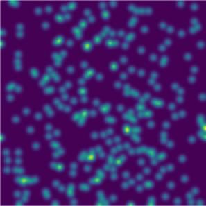
+
                                         CC              CC

                                   CC
                                                                            +   Sum           SeLu

        (a) Simple U-Net with contextual convolutions.                     (b) Contextual convolution.

Figure 1: An illustration of the proposed contextual hourglass networks where shortcut connections
between the bottleneck and later representations are established with the contextual convolution
operation that enforces a spatial alignment of the resulting feature maps.

Under the assumption that both convolutional layers have the same stride of 1 and the same padding
strategy, one movement of the filter bank on T2 to the right (to the bottom) corresponds to bw1 /w2 c
movements to the right (bh1 /h2 c to the bottom) of the filter bank on T1 . Figure 1(a) illustrates the
addition of contextual convolutions to an hourglass type network. For the sake of simplicity, we
only depict the height and depth of the layers’ feature maps. A contextual convolution connects the
bottleneck representations with later layers in the network. The crucial property of the contextual
convolutions is the spatial alignment between the resulting feature maps. Figure 1(b) illustrates the
entanglement of movements of the filter bank on two tensors of different sizes. A movement on
the spatielly more extensive tensor corresponds to a fraction of a movement on the smaller tensor.
We obtained good results with a summation operation and the SeLu activation function. Note that
contectual convolutions can be added to hourglass architectures such as the U-Net [7], V-Net [6], and
the Tiramisu net [3].

3     Experimental Evaluation
3.1   Image Segmentation

We perform experiments on the EM segmentation challenge data set of ISBI 2012. The dataset is
composed of 60 grayscale images of 512 × 512 pixels. There are 30 labeled and 30 unlabeled images.
We trained the networks parameters by randomly sampling 25 labeled images for training and 5 for
validating. Finally, we segmented the 30 unlabeled test images and obtained the resulst by sending
those to the organizers of the challenge. We compare the proposed contextual hourglass networks
with the Tiramisu and U-Net. To ensure a fair comparison we also use the SeLu activation and the
exact same number of layers for the U-Net. We refer to the contextual hourglass architecture as
the “Contextual U-Net.” All models are trained under the same conditions. We randomly initialize
all the weights with the Xavier method [1], alternatively, and with a similar performance, we have
also tried He-Uniform [2]. During the training we optimize the categorical cross entropy loss. The
training strategy consists of two parts. In the first part, we train on augmented the data by performing
randomly distortions. In the second step, we fine tune the models for the nondistorted data. On
each part the models are trained until convergence. Table 1 lists the results. The contextual U-Net
significantly outperforms the other networks showing that the contextual convolutions lead to a
significant improvement over the U-Net architecture. Figure 2(a) depicts some qualitative result on
the validation set.
                                  Table 1: ISBI results on the test set.
                     Method               Rand Score Thin     Information Score Thin
                     Tiramisu-103 [3]          0.7628                0.9165
                     U-Net [7]                 0.8737                0.9594
                     Contextual U-Net          0.9366                0.9737

                                                    2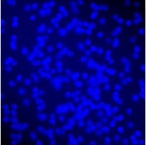
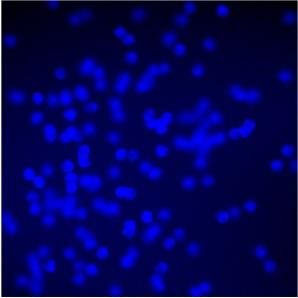
Input
Input
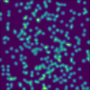
Count: 104.0 Count: 156.0 Count: 292.0
Ground Truth
Ground Truth
Count: 101.1 Count: 158.4 Count: 287.7
Prediction
Prediction
(a) ISBI data set (b) Cell counting data set
Figure 2: Qualitative results for the datasets. Predictions are generated by the contextual U-net.
3.2 Object Counting
We apply the proposed model class to the different problem of cell counting. For this task, we use the
simulated fluorescence microscope images of [4]. We followed the exact same experimental setup as
in previous work [5]. The dataset consists of 200 images. We used the first 32 images for training,
the 68 following images for validation, and the last 100 images for testing. We used a simplified
variant of the contextual U-Net with 3 encoding and 3 decoding steps and set the number of base
filters to 24. We used the mean squared difference as loss function. We train our model from scratch
by initialing its weights with the Xavier algorithm. We perform data augmentations such as random
perturbations and the network is trained until convergence. Table 2 shows the mean absolute error
for N training images. Despite the reduced amount of training data, the proposed model achieve a
competitive performance compared with the current state-of-the-art. In Figure 2(b) we present some
qualitative results.
Table 2: Cell counting results.
Method N=1 N=2 N=4 N=8 N = 16 N = 32
Linear regression [5] 67.3 ± 25.2 37.7 ± 14.0 16.7 ± 3.1 8.8 ± 1.5 6.4 ± 0.7 5.9 ± 0.5
Detection [5] 28.0 ± 20.6 20.8 ± 5.8 13.6 ± 1.5 10.2 ± 1.9 10.4 ± 1.2 8.5 ± 0.5
MESA [5] 9.5 ± 6.1 6.3 ± 1.2 4.9 ± 0.6 4.9 ± 0.7 3.8 ± 0.2 3.5 ± 0.2
Contextual U-Net 6.5 6.5 3.8 3.8 5.2 4.4
References
[1] X. Glorot and Y. Bengio. Understanding the difficulty of training deep feedforward neural
networks. In AISTATS, 2010.
[2] K. He, X. Zhang, S. Ren, and J. Sun. Delving deep into rectifiers: Surpassing human-level
performance on imagenet classification. In ICCV, December 2015.
[3] S. Jégou, M. Drozdzal, D. Vázquez, A. Romero, and Y. Bengio. The one hundred layers tiramisu:
Fully convolutional densenets for semantic segmentation. In CVPR Workshops„ year = 2017.
[4] A. Lehmussola, P. Ruusuvuori, J. Selinummi, H. Huttunen, and O. Yli-Harja. Computational
framework for simulating fluorescence microscope images with cell populations. IEEE Trans.
Med. Imaging, 26(7):1010–1016, 2007.
[5] V. Lempitsky and A. Zisserman. Learning to count objects in images. In NIPS, 2010.
[6] F. Milletari, N. Navab, and S. Ahmadi. V-net: Fully convolutional neural networks for volumetric
medical image segmentation. CoRR, abs/1606.04797, 2016.
[7] O. Ronneberger, P. Fischer, and T. Brox. U-net: Convolutional networks for biomedical image
segmentation. In MICCAI, 2015.
3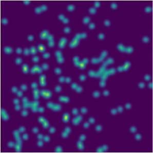
You can also read