Controlling the Global Mean Temperature by Decarbonization - 物理化学学报
←
→
Page content transcription
If your browser does not render page correctly, please read the page content below
物 理 化 学 学 报
                                        Acta Phys. -Chim. Sin. 2021, 37 (5), 2008066 (1 of 7)

[Article]                                         doi: 10.3866/PKU.WHXB202008066                                         www.whxb.pku.edu.cn

Controlling the Global Mean Temperature by Decarbonization
Frits Mathias Dautzenberg 1,*, Yong Lu 2, Bin Xu 3
1 Serenix Corporation, 5632 Coppervein Street, Fort Collins, CO 80528, USA.
2 Shanghai Key Laboratory of Green Chemistry and Chemical Processes, School of Chemistry and Molecular Engineering, East
  China Normal University, Shanghai 200062, China.
3 ECO Zhuo Xin Energy-Saving Technology (Shanghai) Company Limited, Shanghai 201109, China.

Abstract: Establishing a reliable method to predict the global mean
temperature (Te) is of great importance because CO2 reduction activities
require political and global cooperation and significant financial resources.
The current climate models all seem to predict that the earth’s temperature
will continue to increase, mainly based on the assumption that CO2 emissions
cannot be lowered significantly in the foreseeable future. Given the earth’s
multifactor climate system, attributing atmospheric CO2 as the only cause for
the observed temperature anomaly is most likely an oversimplification; the
presence of water (H2O) in the atmosphere should at least be considered. As
such, Te is determined by atmospheric water content controlled by solar
activity, along with anthropogenic CO2 activities. It is possible that the
anthropogenic CO2 activities can be reduced in the future. Based on temperature measurements and thermodynamic data,
a new model for predicting Te has been developed. Using this model, past, current, and future CO2 and H2O data can be
analyzed and the associated Te calculated. This new, esoteric approach is more accurate than various other models, but
has not been reported in the open literature. According to this model, by 2050, Te may increase to 15.5 °C under “business-
as-usual” emissions. By applying a reasonable green technology activity scenario, Te may be reduced to approximately
14.2 °C. To achieve CO2 reductions, the scenario described herein predicts a CO2 reduction potential of 513 gigatons in
30 years. This proposed scenario includes various CO2 reduction activities, carbon capturing technology, mineralization,
and bio-char production; the most important CO2 reductions by 2050 are expected to be achieved mainly in the electricity,
agriculture, and transportation sectors. Other more aggressive and plausible drawdown scenarios have been analyzed as
well, yielding CO2 reduction potentials of 1051 and 1747 gigatons, respectively, in 30 years, but they may reduce global
food production. It is emphasized that the causes and predictions of the global warming trend should be regarded as open
scientific questions because several details concerning the physical processes associated with global warming remain
uncertain. For example, the role of solar activities coupled with Milankovitch cycles are not yet fully understood. In addition,
other factors, such as ocean CO2 uptake and volcanic activity, may not be negligible.

Key Words:        Calculation method for global mean temperature; CO2 in the atmosphere;                           Water in the atmosphere;
                  Global warming; CO2 reduction

Received: August 23, 2020; Revised: September 16, 2020; Accepted: September 18, 2020; Published online: September 21, 2020.
*
 Corresponding author. Email: fritsd@serenixcorp.com.
                                               © Editorial office of Acta Physico-Chimica Sinica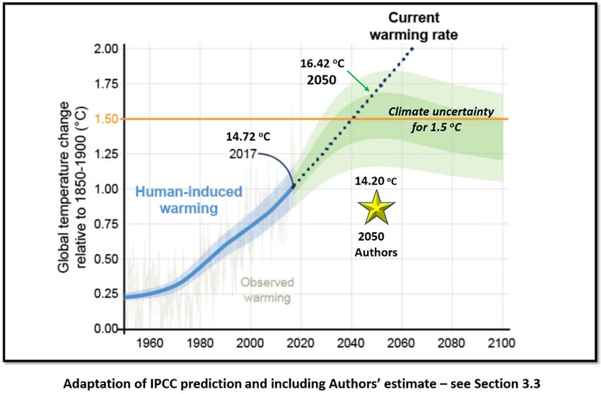
物理化学学报                Acta Phys. -Chim. Sin. 2021, 37 (5), 2008066 (2 of 7)

通过脱碳控制全球平均温度
Frits Mathias Dautzenberg 1,*,路勇 2,徐彬 3
1   Serenix Corporation, 5632 Coppervein Street, Fort Collins, CO 80528, USA.
2   华东师范大学, 化学与分子工程学院,上海市绿色化学与化工过程绿色化重点实验室,上海 200062
3   易高卓新节能技术(上海)有限公司,上海 201109

摘要:建立能可靠预测全球平均温度(Te)的方法,对于寻求政治和全球合作以及大量财政资源来推动CO2减排至关重要。
基于可预见的若干年内CO2排放量不能显著降低这一假设,目前的气候模型似乎都预测Te将会持续上升。然而,将大气
中的CO2作为多因素地球气候系统的唯一变量,来关联观察到的温度异常,很可能过于简单化了,因为大气中H2O的存
在是至少应该要考虑的。受控于太阳活动的大气H2O含量是Te的首要决定因素,其次才是与人类活动相关的CO2排放,而CO2
排放将来可能降低。基于地球平均温度观测值和热力学数据,建立了新的预测模型。应用该模型方程,可以分析过去、
当前和未来大气中CO2和H2O含量并可计算出相应的Te。这是一个还未见公开报道的、更精确的模型。本模型预测,依
据将较基准情景(business-as-usual,BAU),到2050年Te可能上升至15.5 °C;通过合理的绿色技术行动方案,Te可能降
至约14.2 °C,预测未来30年CO2可减排513千兆吨。绿色技术应用场景包括诸如各种CO2减排行动,碳捕获,矿化以及
生物碳生产等,其中至2050年CO2减排的主要贡献将来自于电力、农业和运输行业。另外,也对更激进的Plausible和
Drawdown方案进行了分析,预测未来30年CO2可分别减排1051和1747千兆吨,但这些方案可能会减少全球粮食生产。
要强调的是,全球变暖的成因和预测应该视为开放的科学问题,因为涉及与全球变暖相关的物理过程的多个问题仍然无解。
例如,太阳活动耦合米兰科维奇(Milankovitch)循环扮演的角色就没有完全理解。还有,海洋对CO2的吸收和火山活动等
其他因素的影响,可能无法忽略。

关键词:全球平均温度计算方法;大气CO2含量;大气H2O含量;全球变暖;CO2减排
中图分类号:O642

1     Introduction                                                   new model must also be consistent with thermodynamic
   Many climate models have been developed, based on                 calculations of the atmospheric energy balance. We also like to
mathematical computer simulations of many factors such as the        show how the earth’s temperature may be decreased by certain
temperature of the atmosphere, the oceans and the land surface       reasonable CO2 reduction activities. Other climate change events
and activities on the sun and other factors. These factors all       not caused by the Te have not be the objective of this paper.
interact and are important to determine the average mean world
temperature (Te) and other events related to the earth’s climate.    2   Data and methods
Many scientists legitimately have wondered how accurately            2.1 Global warming
these climate models can predict earth’s future Te. A recent study      Fig. 1 shows the Te (in blue) from 1850–2020. In brown, we
by environmental scientists from Berkeley 1 has shown that the       indicate what the Te would have been if the temperature increase
climate models published during the past five decades have           were 0.0025 °C per year, which was the case from 1600 till 2000,
skillfully described Te changes, with most examined models           according to Table 1. At this moment, the measured temperature
showing global temperature warming consistent with                   is about 1 °C higher than the brown temperature. If this trend
observations, particularly when mismatches between model-            would continue (see Fig. 2), the Te would be 16.4 °C by 2050,
calculated and observationally estimated were taken into
account. Regarding the future Te, the current climate models all
seem to predict that the earth’s temperature will continue to
increase mainly assuming that CO2 emissions cannot be lowered
significantly in the foreseeable years.
   In this paper, we will analyze observational data regarding
global warming. Using readily available data, a simple
calculation method for the Te is proposed since other models
published in the literature are not accurately predicting the
future. This new proposed model should take into consideration
the water in the atmosphere and anthropogenic CO2. The simple         Fig. 1 The Te in °C in the past 140 years, based on data from Refs. 2–4.
物理化学学报 Acta Phys. -Chim. Sin. 2021, 37 (5), 2008066 (3 of 7)
Table 1 Global temperature increase per year, including data from
the National Aeronautics and Space Administration (NASA) and the
Goddard Institute for Space Studies (GISS).
Years T T/year T/100 year
Core Ice 10000 11 0.0011 0.11
1600–2000 400 1.0 0.0025 0.25
1910–2020 110 1.4 0.0127 1.27
1980–2019 39 0.9 0.0231 2.31
Fig. 3 Calculating a and b coefficients from experimental data.
Ref. 3 (NASA, GISS), Ref. 4 (Buis), Ref. 5 (Moore), Ref. 6 (Spencer), and
Ref. 7 (Petit).
only needs the heat of formation divided by heat capacity Cp for
calculating b. The thermodynamic calculations for H2O and CO2
are shown in Table 2 and Table 3. The a and b values using
thermodynamics are close to the experimental data, with a delta
of less than 2%.
The value of b can be used to establish the CO2 sensitivity as
a function of CO2 increases in the atmosphere. Starting with a
CO2 level is 280 (× 10−6(v)) in 1870 and 410 (× 10−6(v)) in 2019,
the CO2 sensitivity becomes (1.065 × 10−2) × (410 − 280) =
1.38 °C. If the CO2 doubled to 560 (× 10−6(v)), the CO2
sensitivity would become 2.98 °C, in line with recently reported
data in the literature with values from 2.2–3.4 °C 12. On this
Fig. 2 Expected global temperature change according to the basis, we estimated that the CO2 in the atmosphere should not
IPCC 2 and the author’s scenario. pass beyond 440 (× 10−6(v)) by 2050 if one aims at a maximum
temperature increase of 1.5 °C in the future. It will be shown in
Section 3.2 how this stringent objective is achievable.
and by 2100, the Te would be 19.0 °C 2. It becomes clear that the
current global temperature increases of 0.0231 °C/year (from
1980 till 2019, see Table 1) is considerably higher than ever Table 2 Thermodynamic calculations * of a coefficient.
experienced on earth. However, we like to understand the causes T/°C T/K ΔHf/(kJ·mol−1) ΔHvap/(kJ·mol−1) Cp/(kJ·mol−1·K−1) a/°C/(10−6(v))
of the observed increase of the Te, on a solid scientific basis. 25.00 298.15 −241.89 44.54 0.07537 2.6182 × 10⁻³
2.2 Global temperature as a function of water vapor 13.50 286.65 −242.27 43.98 0.07560 2.6227 × 10⁻³
and CO2 in the atmosphere 13.95 287.10 −242.25 44.01 0.07559 2.6226 × 10⁻³
The Te is related to the amount of water in the atmosphere 14.50 287.65 −242.23 44.03 0.07558 2.6225 × 10⁻³
(largely controlled by solar irradiation 8,9) and added CO2. The 15.10 288.25 −242.21 44.06 0.07556 2.6224 × 10⁻³
amount of CO2 in the atmosphere is currently measured daily. 15.50 288.65 −242.20 44.08 0.07555 2.6223 × 10⁻³
That has not been the case for water vapor in the atmosphere. 16.00 289.15 −242.18 44.10 0.07554 2.6221 × 10⁻³
However, data from the National Aeronautics and Space
16.50 289.65 −242.17 44.13 0.07553 2.6220 × 10⁻³
Administration (NASA) covering global precipitation (in mm
17.00 290.15 −242.15 44.15 0.07552 2.6219 × 10⁻³
per day) from 1900 till 2000 allow us to estimate the water *
Thermodynamic data in Refs. 10, 11.
content of the atmosphere since the residence of rain is known
Table 3 Thermodynamic calculations * of b coefficient.
to be approximately 9 days.
Using the observed CO2 and water data of the earth’s T/°C T/K ΔHf/(kJ·mol−1) Cp/(kJ·mol−1·K−1) b/°C/(10−6(v))
atmosphere in 1970 and 2019 and the measured Te at those times 13.50 286.65 −393.95 37.40 1.0532 × 10⁻²
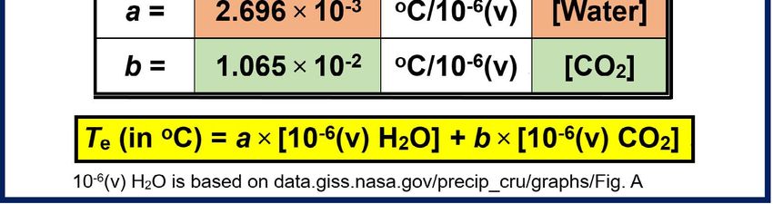
(see Fig. 3), one can calculate two coefficients, one for water a 13.95 287.10 −393.93 37.42 1.0526 × 10⁻²
and one for CO2 b according to the following equation.
14.50 287.65 −393.91 37.45 1.0519 × 10⁻²
Te (in °C) = a × [10−6(v) H2O] + b × [10−6(v) CO2] (1)
The experimental value of a = 2.696 × 10⁻³ in °C/(10−6(v)), 15.10 288.25 −393.89 37.47 1.0511 × 10⁻²
while the value for b =1.065 × 10⁻² in °C/(10−6(v)). 15.50 288.65 −393.88 37.49 1.0506 × 10⁻²
Using thermodynamic data 10,11, one can estimate the value of
16.00 289.15 −393.86 37.51 1.0499 × 10⁻²
a and b. For water, one uses the heat of formation of gaseous
16.50 289.65 −393.84 37.53 1.0493 × 10⁻²
water, minus the heat of vaporization divided by the heat
capacity Cp of liquid water to calculate the coefficient a 17.00 290.15 −393.82 37.56 1.0486 × 10⁻²
in °C/(10−6(v)). Since CO2 is a gas at 13.95 and 15.10 °C, one *
Thermodynamic data in Refs. 10, 11.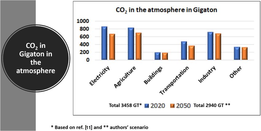
物理化学学报                  Acta Phys. -Chim. Sin. 2021, 37 (5), 2008066 (4 of 7)

3 Results
3.1 Past and future global temperatures using Eq.
       (1)
   In many cases, one measured the Te and the CO2 in 10−6(v).
Fig. 4 shows data for CO2, H2O, and associated Te from 1880 till
2019, using Eq. (1). The observed CO2 and H2O data of 1970
and 2019 were used to establish the a and b coefficients, as
discussed in Section 2.2. The CO2 did increase from 280 (×
10−6(v)) in 1880 to 410 (× 10−6(v)) in 2019 (see Fig. 4). The
concentration of H2O in the atmosphere varied slightly during
this period, which is possibly a natural trend 13, depending on the        Fig. 5 CO2 and H2O in the atmosphere and associated Te in the
absorbed solar radiation. This indicates that, on average, 71% of                             past, current and future.
the observed Te is caused by H2O in the atmosphere, while CO2
contributes 29%.                                                        15.5 °C by 2050 and about 17.0 °C by 2100, extrapolating the Te
   From 1980 to 2019, the delta Te increased from 0.50 °C to            increased from 1980–2019 by 0.0231 °C/year (see Table 1).
1.44 °C, relative to maintaining CO2 at 280 (× 10−6(v)), as in          These Te estimates are lower than mentioned above in section
1870. The delta Te increase due to higher CO2 was, therefore,           2.1 based on IPCC data, but it is more important that we agree
0.024 °C per year from 1980 to 2019 (see Table 1), which is an          with many scientists that everything should be done to keep the
alarming increase, according to the authors of the                      Te increase at about 1.5–2.0 °C, including most of the
Intergovernmental Panel on Climate Change (IPCC) reports 2.             participants of the IPCC 2. However, it is well known that not
   As shown in references 14–17, the earth’s temperatures in the        everybody agrees with the IPCC objective (see, e.g., Refs. 5, 6,
past have been significantly higher than the current Te, while the      18, 21 as typical examples).
levels of CO2 have been higher as well as lower than the current           The most effective way to manage anthropologic CO2
CO2 level at 410 (× 10−6(v)) (see Fig. 5). We, therefore, conclude      emissions is to avoid the formation of CO2. Furthermore, carbon-
that there is no clear correlation between the Te of the earth and      neutral technologies may assist in greening the world. Also,
the CO2 in the atmosphere, as noted by other scientists as well 6,18.   photosynthesis is an essential natural method to reduce CO2 from
   In 1998, 24.4 gigatons of CO2 was added to the atmosphere,           the atmosphere, and technologies that remove CO2 from the
increasing to 36.6 gigatons in 2018 19. As a result, the                atmosphere may also become viable in the future. In the
atmosphere contained 3120 gigatons CO2 in 1998 and 3450                 following paragraphs, we will present summaries of what can be
gigatons in 2018. That corresponds to a CO2 residence time of           achieved.
about 30 years, in line with various papers in the literature, e.g.,    3.2.1 Electrical power generation
Ref. 20. Consequently, only a fraction of the emitted CO2                  It is apparent that CO2 reduction options for electrical power
remains in the atmosphere (equal to 0.918), while the remaining         generation are being pursued around the world. By 2050, we
CO2 will be absorbed by oceans, seas, and land, including               estimate that 215 gigatons of CO2 can be avoided mainly by
photosynthesis activities.                                              applying wind and solar technology.
3.2 Approaches to decrease CO2 in the atmosphere                        3.2.2 Agriculture including forestry
   Using a similar approach for calculating the CO2 in the                 CO2 reduction in the agriculture sector is also possible 22,23. In
atmosphere from 1998 till 2018 (see Section 3.1) and applying a         the next 30 years 471.5 gigatons of CO2 emissions could be
“business-as-usable” scenario, we estimate that the Te could be         avoided. Forestry management, new agriculture technologies,
                                                                        and reducing food waste are likely the key areas with the most
                                                                        significant impact. Around the world, large scale reforestation
                                                                        projects are in progress, like in China, Brazil, USA, Morocco,
                                                                        and other countries
                                                                        3.2.3 Building
                                                                           Better maintenance of air conditioning equipment could
                                                                        potentially reduce CO2 emissions by 89.4 gigatons between 2020
                                                                        and 2050 22. Additionally, another 54.5 gigatons CO2 reductions
                                                                        are possible using, for instance, district heating, better insulation,
                                                                        and LED lighting.
                                                                        3.2.4 Transportation
                                                                           The transportation sector can potentially reduce CO2
    Fig. 4 CO2 and H2O in the atmosphere and associated Te from         emissions by 134 gigatons during the period from 2020 to 2050.
                           1880 till 2019.                              This may be achieved using a variety of technologies. Around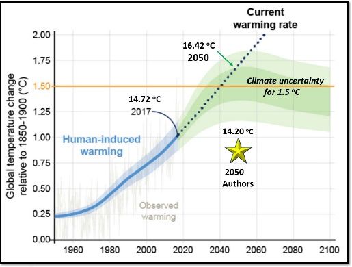
物理化学学报 Acta Phys. -Chim. Sin. 2021, 37 (5), 2008066 (5 of 7)
the world, hydrogen fueled cars, electric cars, hybrid cars and geological formations and reservoirs. However, the risk remains
mass transportation are already actively pursued and improved that potentially suitable reservoirs may turn out to be
ships, trucks, and airplanes will follow as well. Biomass can be insufficient, uneconomic, or impractical 27.
converted to transportation fuels, enabling carbon neutral Carbon capture and mineral carbonation (CCMC), also called
recycling 24,25. CO2 mineralization, has been identified by the IPCC as a
3.2.5 Industry possible promising additional technology to remove CO2 from
In the industry sector, fuels, and chemicals from sustainable the atmosphere. CCMC is a process whereby CO2 is chemically
resources 24 can lead to reductions in CO2 emissions. Biomass, reacted with calcium- and/or magnesium-containing minerals to
municipal solid waste, and other carbon-containing streams can form stable carbonate materials which do not incur any long-
be used to produce bio-SNG, bio-jet fuel, green methanol, and term liability or monitoring commitments. CCMC is highly
green ammonia 25. It may take some time to transform the verifiable and permanent in nature. Companies are pursuing
industry sector to greener technologies, but several companies CCMC, and demonstration pilot plants have already been in
are already working on this. operation 28. Australia recently discovered large deposits of
3.2.6 Other CO2 reduction methods halloysite-kaolin clay that can be used for CCMC 29.
Education and family planning are highlighted to reverse the 3.2.10 Direct air capture of CO2
global temperature increase 25, reducing CO2 emissions by 109.2 Biochar plus CO2 mineralization can potentially remove about
Gigatons during the next 30 years. One hopes that with education 78 gigatons of CO2 in 30 years, as estimated in Ref. 22. By 2050,
and family planning, the total world population will not increase direct air capture of CO2 could become an additional viable
as fast as projected. technology, if the captured CO2 is used for CCS and/or CCMC.
In addition to the methods reviewed above, one can remove 3.2.11 Geoengineering
CO2 from the atmosphere to lower the Te. The following Star Technology and Research 30 has designed a system of
approaches may be suitable. space mirrors that blocks sunlight from reaching the earth and
3.2.7 Photosynthesis provides another source of clean energy for the earth. These
Photosynthesis is a natural way to remove CO2 from the spacecraft mirrors are remotely controlled and equipped with
atmosphere. This requires that the atmosphere contains at least solar panels that collect some of the sunlight and send the
150 (× 10−6(v)) CO2 with an optimum CO2 level of 1500 (× captured energy back down to earth. However, geoengineering
10−6(v)). For this reason, farmers and gardeners add CO2 to their has many potential pitfalls that have not made it popular with
greenhouses. scientists, whose climate platforms focus instead on ways to
3.2.8 Biochar reduce the earth away from fossil fuels 31.
Biochar is an emerging carbon material derived from 3.3 Applying scenarios to reduce CO2 emissions
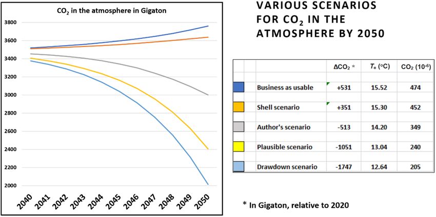
renewable resources. This has triggered great interest in a variety Five scenarios have been developed (see Fig. 6), using similar
of areas, including carbon sequestration and potential soil calculations to assess the CO2 in the atmosphere from 1998 to
amendments 26. Trees and plants do grow faster in sandy soil 2018, shown in Section 3.2. The first scenario, called “Business-
mixed with clay, biochar, and mycorrhizae fungi if one has as-usable” (BAU), extrapolates the current CO2 emissions data 13
enough water. This had been demonstrated successfully, for until 2050, leading to an increase of 531 gigatons CO2 in the
instance, in the Gobi Desert in China and around the Sahara for atmosphere. The Shell scenario 32 is a little better than the BAU
the Great Green Wall initiative. scenario but still increases the CO2 in the atmosphere of 351
3.2.9 CO2 mineralization gigatons. The most aggressive scenarios are called “Plausible”
To date, the most widely accepted method of carbon capture and “Drawdown” based on Ref. 22. The input of 192 well-known
and storage (CCS) is the injection of CO2 into underground environmental experts, scientists, engineers, architects, lawyers
Fig. 6 Various scenarios for CO2 in the atmosphere by 2050.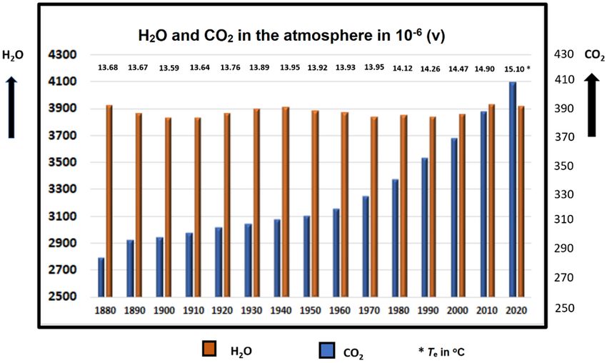
物理化学学报                  Acta Phys. -Chim. Sin. 2021, 37 (5), 2008066 (6 of 7)

                           Fig. 7 CO2 in gigaton in the atmosphere, based on authors’ scenario and data from Ref. 11.

and writers have contributed to the formulation of the Plausible          2 illustrates the expected Te according to the IPCC 2 and the
and Drawdown scenarios. The Plausible scenario is an                      author’s scenario. If “Business as usable” is happening, the IPCC
optimistic, feasible frame work and forecast of CO2 reduction             projects that the Te could increase to 16.4 °C by 2050. Applying
activities that could impact the global climate with a total CO2          the correlations describes in Section 3.2, we estimate that the Te
reduction of 1051 gigatons in 30 years. The Drawdown scenario             may increase to 15.5 °C for a “Business as usable” scenario.
describes the most comprehensive plan to reverse global                   According to the author’s scenario, a Te of 14.2 °C seems to be
warming. It shows what would happen when the more                         achievable by 2050. Using the proposed simple model to
conservative assumptions of the Plausible scenario are removed.           calculate Te may seem to be an oversimplification, since it does
In this case, a total CO2 reduction of 1747 gigatons in 30 years          not predict other important climate events, which were not part
could be realized. The proposed authors’ scenario is selected as          of the paper’s objective.
an achievable compromise approach, predicting a CO2 reduction                Indeed, several questions regarding physical processes
potential of 513 gigatons. Fig. 6 also lists corresponding global         associated with global warming remain unanswered. That means
Te in °C and the expected CO2 in 10−6(v). The Plausible and the           that the causes and prediction of the global warming trend should
Drawdown scenarios would affect global food production since              be considered as open scientific questions. For instance, the roles
the CO2 would drop to 240 (× 10−6(v)) and 205 (× 10−6(v)), lower          of sun activities coupled with Milankovitch cycles, are not fully
than in 1850.                                                             understood yet. Also, other factors like ocean CO2 uptake and
   The anthropologic CO2 emission in 2020 is estimated to lead            volcanic activities, may not be negligible.
to 3458 gigatons of CO2 in the atmosphere, applying the trends               Basing the multi-factor earth’s climate system to CO2 in the
shown on Ref. 19. According to the author’s scenario, the CO2             atmosphere as the only variable causing the observed
in the atmosphere would reduce to 2945 gigatons. The
                                                                          temperature anomaly is most likely an oversimplification,
distribution of this amount by sectors of activity is shown in Fig.
                                                                          because one should at least consider the presence of water in the
7. The data indicates that relative to 2020, the most important
                                                                          atmosphere. That does not mean that efforts to lower CO2
CO2 reductions by 2050 are expected to be achieved mainly in
                                                                          emissions should not be pursued because getting to a fossil-free
the electricity, agriculture, and transportation sectors.
                                                                          world is ultimately unavoidable and will create progress in many
                                                                          ways.
4 Conclusion and discussion
   It is a fact that the mean temperature of the earth has been
                                                                          Conflict of interest:           The authors declare that they have no
increasing slightly during the past 60 years, which is supported
                                                                          conflict of interest.
by numerous data. Referring to Section 3.1, the a and b
coefficients are based on observational data such as the Te, the
CO2 in the atmosphere, and water in the atmosphere derived                References
from rainfall records. The thermodynamic calculated a and b                 (1) Hausfather, Z.; Drake, H. F.; Abott, T.; Schmidt, G. A. Geophys. Res.
coefficients are in line with the experimental values.                           Lett. 2020, 47 (1), e2019GL085378. doi: 10.1029/2019GL085378
Furthermore, the 0.918 CO2 decrease rate per year used in                   (2) Intergovernmental Panel on Climate Change (IPCC) Reports, 1990–
Section 3.1 shows that CO2 remains in the atmosphere for many
                                                                                 2019. https://www.ipcc.ch (accessed on Sep. 18, 2020).
years, while water in the atmosphere only stays about 9 days.
                                                                            (3) GISS Surface Temperature Analysis (GISTEMP v4), version 4, 2019.
The amount of water in the atmosphere is, however, more
dominant in terms of the earth’s temperature than the                            https://data.giss.nasa.gov/gistemp (accessed on Sep. 18 2020).

contribution of CO2. The amount of water hardly changed from                (4) Buis, A. Study conforms climate models are getting future warming
1850 till 2020, independent of the increasing CO2 amount. Fig.                   projections right. https://climate.nasa.gov/news/2943/study-confirms-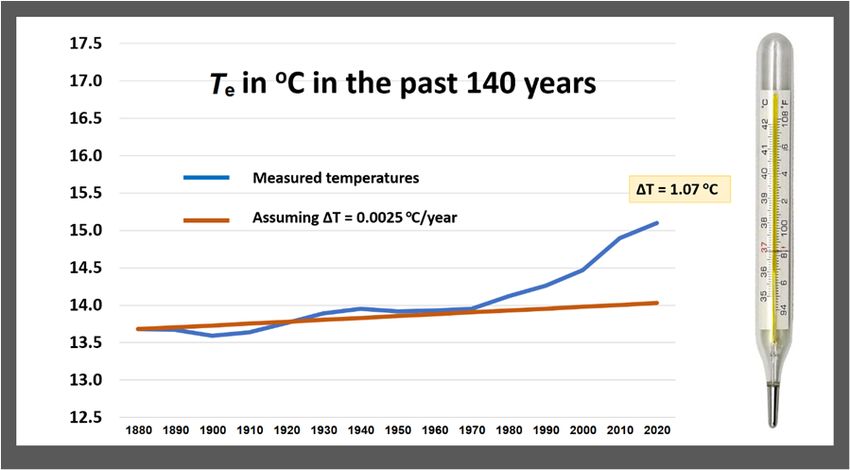
物理化学学报                     Acta Phys. -Chim. Sin. 2021, 37 (5), 2008066 (7 of 7)

      climate-models-are-getting-future-warming-projections-right/                    (accessed on Sep. 18, 2020).

      (accessed on Sep. 18 2020).                                               (20) Abbot, J.; Marohasy, J. Geo. Res. J. 2017, 14, 36.

 (5) Moore, P. A. Confessions of a Greenpeace Dropout; Beatty Street                  doi: 10.1016/j.grj.2017.08.001

      Publishing Inc.: Vancouver, BC, Canada, 2013.                             (21) https://www.therightinsight.org/Patrick-Moore-Should-We-

 (6) Spencer, R. W. The Greatest Global Warming Blunder: How Mother                   Celebrate-CO2 (accessed on Sep. 18, 2020).

      Nature Fooled the World’s Top Climate Scientists; Encounter Books:        (22) Hawken, P. Drawdown-The Most Comprehensive Plan Ever

      New York, NY, USA, 2010.                                                        Proposed to Reverse Global Warming; Penguin Books, New York,

 (7) Petit, J. R.; Jouzel, J.; Raynaud, D.; Barkov, N. I.; Barnola, J. -M.;           NY, USA, 2017.

      Basile, I.; Bender, M.; Chappellaz, J.; Davis, M.; Delaygue, G.; et al.   (23) Henson, R. The Thinking Person’s Guide to Climate Change, 2nd ed.;

      Nature 1999, 399 (6735), 429. doi: 10.1038/20859                                The American Meteorological Society: Boston, MA, USA, 2019.

 (8) Bohren, C. F.; Clothiaux, E. E. Fundamentals of Atmospheric                (24) Vertes, A.; Qureshi, N.; Yukawa, H.; Blaschek, H. Biomass to

      Radiation: An Introduction with 400 Problems; Wiley-VCH Verlag                  Biofuels: Strategies for Global Industries. John Wiley & Sons LTD.:

      GmbH & Co. KGaA: Weinheim, Germany, 2006.                                       Chicher, West Sussex, UK, 2010.

 (9) www.geo.utexas.edu/courses/387H/Lectures/chap2.pdf (accessed on            (25) Anastassiadis, S. G. World J. Bio. Biotechnol. 2016, 1 (1), 1.

      Sep. 18 2020).                                                                  doi: 10.33865/wjb.001.01.0002

(10) https://www.nist.gov/publications/web-thermo-tables-line-version-          (26) Han, L.; Ro, K. S; Sun, K.; Sun, H.; Wang, Z.; Libra, J. A.; Xing, B.

      trc-thermodynamics-table (accessed on Sep. 18, 2020).                           Environ. Sci. Technol. 2016, 50 (24), 13274.

(11) Yaws, C. L. Chemical Properties Handbook; McGraw-Hill: New                       doi: 10.1021/acs.est.6b02401

      York, NY, USA, 1999; p. 291 and p. 310.                                   (27) Doucet, F. J. Scoping Study on CO2 Mineralization Technologies.

(12) Cox, P. M.; Huntingford, C.; Williamson, M. S. Nature 2018, 533                  Report No. CGS-2011-007-Prepared for South African Centre for

      (7688), 319. doi: 10.1038/nature25450                                           Carbon Capture and Storage, 2011.

(13) Deser, C. Making Sense of Climate Projections. Lecture at the              (28) Xie, H.; Yue, H.; Zhu, J.; Liang, B.; Li, C.; Wang, Y.; Xie, L.; Zhou,

      University of Washington, Department of Atmospheric Sciences:                   X. Engineering 2015, 1 (1), 150. doi: 10.15302/J-ENG-2015017

      Seattle, WA, USA, 2019.                                                   (29) https://www.theleadsouthaustria.com.au, Willis, B. Global carbon

(14) http://www.scotese.com/earth.htm. (accessed on Sep. 18 2020)                     capture potential for rare nanoparticles, 2020, March 24 (accessed on

(15) Ruddiman, W. F. Earth’s Climate: Past and Future, 3rd ed.; W.H.                  Sep. 18, 2020).

      Freeman & Sons: New York, NY, USA, 2013.                                  (30) Dean, C. Expert Discuss Engineering Feats, Like Space Mirrors to

(16) Pagani, M.; Zachos, J. C.; Freeman, K. H.; Tipple, B.; Bohaty, S.                Slow Climate Change; The New York Times: New York, NY, USA,

      Science 2005, 309 (5734), 600. doi: 10.1126/science.1110063                     Nov. 10, 2007.

(17) https://www.sciencemag.org/news/2019/05/500-million-year-survey-           (31) Gramling, C. In a Climate Crisis, Is Geoengineering Worth the Risks?

      earths-climate-reveals-dire-warning-humanity (accessed on Sep. 18               Science News; Society for Science & the Public: Washington DC,

      2020).                                                                          USA, Oct. 6, 2019.

(18) Moore, P. A. Climate Realism. Presentation at the Climate Realism          (32) www.shell.com/energy-and-innovation/the-energy-

      seminar, Toronto, Canada, October, 2019.                                        future/scenarios/shell-scenario-sky.html (accessed on Sep. 18, 2020).

(19) https://ourworldindata.org/CO2-and-other-greenhouse-gas-emissions
You can also read