COVID-19 lockdown only partially alleviates health impacts of air pollution in Northern Italy - OSF
←
→
Page content transcription
If your browser does not render page correctly, please read the page content below
COVID-19 lockdown only partially alleviates health impacts of air
                                                                                ∗
                                   pollution in Northern Italy
   Francesco Granella†a,b , Lara Aleluia Reisb , Valentina Bosettia,b and Massimo Tavonib,c

                                             a
                                       Bocconi University
               b
                   RFF-CMCC European Institute on Economics and the Environment
                                    c
                                      Politecnico di Milano

                                                    Abstract

             The harsh lockdown measures that marked the response to the COVID-19 outbreak in the
         Italian region of Lombardy provides a unique natural experiment for assessing the sensitivity of
         local air pollution to emissions. However, evaluating the pollution benefits of the lockdown is
         complicated by confounding factors such as variations in weather. We use a machine learning
         algorithm that does not require identifying comparable but unaffected regions while addressing
         the effect of weather. We show that the lockdown, albeit virtually halting most human ac-
         tivities, reduced background concentrations of PM2.5 by 3.84 µg/m3 (16%) and NO2 by 10.85
         µg/m3 (33%). Improved air quality has saved at least 11% of the years of life lost and 19%
         of the premature deaths attributable to COVID-19 in the region. Although air pollution has
         significantly decreased, it has often remained above safety thresholds. The analysis highlights
         the diversity of air pollution sources and the need for an expansive policy response.

         Keywords: Air pollution, COVID-19, machine learning, health

   ∗
       We thank participants to the RFF-CMCC webinar for useful comments and Guido Lanzani for valuable discus-
sions. We declare no conflicting interests. This research received no specific grant from any funding agency in the
public, commercial, or not-for-profit sectors.
  †
    Corresponding author, francesco.granella@unibocconi.it.

                                                        1
1    Introduction

Exposure to airborne pollutants is detrimental to human health. Fine particulate matter (PM2.5 )

increases mortality rates and hospitalizations due to respiratory and cardiovascular disease (Pope

and Dockery 2006; Ebenstein et al. 2017; Deryugina et al. 2019). Additionally, it leads to a decline

in physical and cognitive productivity (Graff Zivin and Neidell 2012; Ebenstein et al. 2016; Zhang

et al. 2018; He et al. 2019; Kahn and Li 2020). Similarly, exposure to nitrogen dioxide (NO2 ) leads

to an increase in hospital admissions and premature mortality (Mills et al. 2015; Amini et al. 2019;

Duan et al. 2019).

    In general, the design of effective pollution abatement policies requires mapping reductions in

emissions to reductions in concentrations. However, the processes of formation, transport, and

dispersion of pollutants are complex phenomena, introducing considerable ex-ante uncertainty on

the effect of policies on air quality. Moreover, ex-post evaluation studies need to address the

confounding effect of idiosyncratic weather, a significant driver of pollutant concentrations.

    In this paper, we provide novel evidence on the change in concentrations of PM2.5 and NO2

following a heterogeneous reduction in emissions across different sources. Specifically, we exploit

the dramatic reduction in mobility and economic activity in Italy in response to the COVID-19

outbreak from late February to early May.

    We provide causal estimates of the change in PM2.5 and NO2 over more than two months for

Lombardy, one of the most polluted regions among Organisation for Economic Co-operation and

Development countries. Lombardy is also one of the first areas outside China that imposed a strict

lockdown. Using a machine learning algorithm, we address the confounding effect of weather and

build a counterfactual of the pollution concentrations that would have occurred if the COVID-19

pandemic had not broken out, and no lockdown had been implemented. Finally, we compute the

years of life saved and the number of avoided premature deaths by the improvement in air quality,

and compare these numbers against the years of life lost and premature deaths due to COVID-19

in the region over the same period.

    Ex-post studies can provide valuable estimates of the sensitivity of concentrations to emissions.

However, a host of confounding factors can seriously hinder causal inference. In particular, the

                                                  2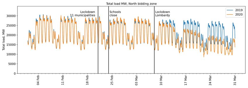
concentration of airborne pollutants is highly dependent on atmospheric conditions. Formation,

transport and dispersion, and even emission of pollutants are directly or indirectly affected by the

weather (Kroll et al. 2020). For instance, severe haze events in Beijing follow periodic cycles gov-

erned by meteorological conditions, especially wind patterns (Guo et al. 2014). Unless confounding

factors as weather are accounted for, the estimated change in concentrations following intervention

is biased, and little is known on the direction of the bias.

   A common approach to ex-post evaluation of pollution control policies is comparing treated and

control units (e.g., He et al. (2020) and Cole et al. (2020) for the case of COVID-19 lockdowns).

However, even when the idiosyncratic role of weather has been accounted for, comparable but

untreated units may not always be available. Doubts of spillover effects in control regions could be

raised, even more so considering the ubiquitous adoption of measures to control the spreading of

COVID-19. Finally, the time window between the imposition of restrictive measures in treatment

and control units may not be long enough for policy-relevant results.

   We turn the complex correlation of weather and pollution to our favor, predicting concen-

trations as a sole function of weather variables and season with machine learning. We follow a

simple strategy, similar to Petetin et al. (2020), that does not require identifying comparable but

unaffected regions. For each air pollution monitoring station in the region, we train an extreme

gradient boosting regressor (Friedman 2001), a tree-based machine learning algorithm, over daily

concentrations from 2012 to 2019 and predict concentrations for the first four months of 2020, that

is before and throughout the lockdown. We show in Supplementary information that this approach

is more reliable than linear regression models. To account for any systemic bias in the counterfac-

tual, including inter-annual trends (Silver et al. 2020), we adopt a difference-in-differences strategy.

We identify the average impact of the lockdown on concentrations as the difference between the

prediction error before and during the lockdown.

   We find that, despite the unprecedented halt in mobility and economic activity, the concentra-

tions of major pollutants only partially decreased as a consequence of the lockdown. Background

concentrations of PM2.5 and NO2 decreased by 3.84 µg/m3 (16%) and 10.85 µg/m3 (33%), respec-

                                                   3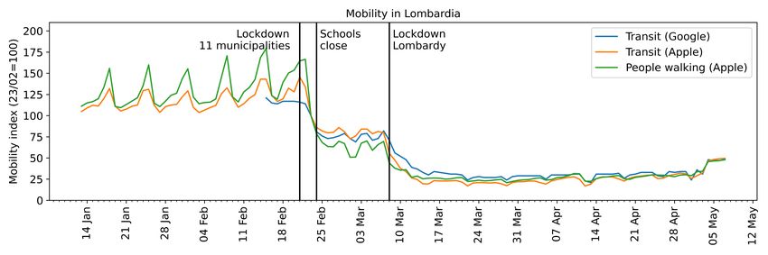
tively. Nonetheless, the improvement in air quality saved at least 11% of the years of life lost and

19% of the premature deaths attributable to COVID-19 in the region during the same period.

2    Sectoral emissions during lockdown

The timing and nature of the lockdown of Lombardy and Italy are discussed in detail in the

Supplementary information. We highlight here two key moments. On February 21, 2020, the

first outbreak of COVID-19 in Italy was identified in the south of Lombardy. Within 24 hours,

11 municipalities in the region went under strict lockdown: schools were closed, all non-essential

economic activities had to stop, and a stay-at-home order was in place. Teaching activities in the

rest of Lombardy also were suspended. On March 8, authorities extended the lockdown to the rest

of Lombardy; and to the rest of Italy on the following day. Lockdown measures were kept in place

almost unaltered until May 4.

    The progressive spreading of the virus in Northern Italy and the tightening of containment

measures have substantially reduced mobility and economic activity. As mobile phone data reveals,

the movement of individuals in Lombardy has followed a two-step response, following the first

outbreak of COVID-19 cases in lower Lombardy (February 21) and the lockdown of the entire

country (March 9) (Figure 1a). By mid-March, mobility dropped by three-fourths, according to

data compiled by Google and Apple (Google 2020; Apple 2020). Under lockdown, all non-essential

industrial production halted. As a consequence, energy demand in Northern Italy steadily decreased

since March 9, as businesses shut down, bottoming to 50% of pre-lockdown levels after two weeks

(Figure 1b).

    However, not all major sources of emissions, especially those releasing precursors of PM2.5 , have

been affected by restrictions. The lockdown forced most people to home isolation; it is sensible

to hypothesize that emissions from residential buildings increased as a consequence. On the other

hand, emissions from non-residential buildings might have decreased. Although data to confirm

this is lacking, it is plausible that emissions from heating systems have not decreased substantially.

    During the transition between winter and spring, agriculture becomes an important source of

secondary PM2.5 in Lombardy (INEMAR 2017). The dispersal of animal liquids on open fields is

                                                  4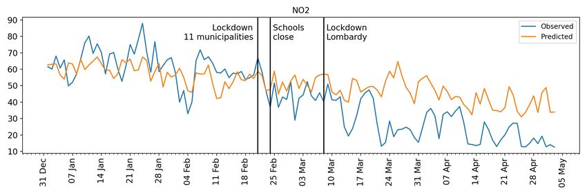
a common (though regulated) practice that releases ammonia in the atmosphere, a precursor to

secondary PM2.5 . Public authorities have not restricted agricultural activities during lockdown in

the interest of securing food supplies. These practices have continued virtually unchanged compared

to previous years (personal exchange with public officials at the regional office for agriculture).

                                                 (a)

                                                 (b)

Figure 1: Proxies of sectoral emissions. a, Mobility indices for Milan Lombardy based on
mobile phone data. Indices equal 100 on February 23. Source: Google (2020); Apple (2020). b,
Total load of energy demand in Northern Italy in MW, 2019 vs 2010. The time series of 2019 has
been shifted to match the day of the week. Source: TERNA (2020).

3    Methods

To identify the causal effect of the lockdown on concentrations without directly observing emissions,

we build a synthetic counterfactual. We train a machine learning algorithm that can reproduce

                                                  5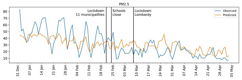
pollution concentrations on a business-as-usual scenario, and then predict concentrations during the

lockdown. The difference between observed concentrations and the counterfactual, or prediction

error, is the effect of the intervention. To account for potential systemic bias in the counterfactual,

we adopt a difference-in-differences strategy. We identify the average impact of the lockdown on

concentrations as the difference between the prediction error before and during the lockdown. This

approach does not require identifying a comparable regions whose concentrations follow a business-

as-usual trend.

      We first assemble a dataset of air pollution, atmospheric conditions, and calendar variables for

the period 2012 to 2020 for the Italian region of Lombardy. Pollution concentrations are measured at

83 monitoring stations. Data on daily minimum and maximum temperature, average wind speed

and wind direction, average relative humidity, daily cumulative precipitation, and atmospheric

soundings come from 227 weather stations

      For every monitoring station, we build the counterfactual using an extreme gradient boosting

regressor, a tree-based model (Friedman 2001).1 Next, monitor by monitor, we train the algorithm

on data from 2012 through 2019 and predict concentrations of PM2.5 and NO2 in 2020. We use

the pre-lockdown period from January 1 to February 22, which has not entered the training set, to

assess the validity of the counterfactual.

      As our ultimate goal is a reliable prediction of pollutant concentrations from January through

early May 2020, cross-validation is performed over four folds, each one consisting of the months from

January to April for 2016, 2017, 2018, and 2019. The more common cross-validation on random

subsamples, or folds, gives equal weight to all seasons. However, with such validation strategy it

cannot be ruled out that an algorithm make good average predictions, while over-predicting in

one season and under-predicting in the opposite one. Suppose, for instance, that the predictions

of a learner are positively biased in spring, negatively biased in fall, and unbiased in winter and

summer. In this case, testing predictions on the pre-lockdown period (in wintertime) does not give

correct estimates of the bias during the lockdown (in springtime). For this reason, we perform
  1
      We use the python package xgboost (Chen and Guestrin 2016).

                                                       6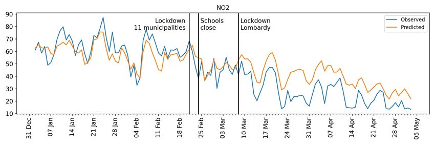
cross-validation over the months for which we want predictions to be reliable. Model parameters

are selected to maximize the cross-validated RMSE.

       The identification strategy relies on two assumptions. First, input variables should not be

themselves affected by the intervention; otherwise, estimated effects will be biased towards zero.

To this end, we exploit the sensitivity of concentrations to meteorological conditions and build the

counterfactual as a sole function of weather and season. While emissions are affected by weather

(e.g., lower emissions from heating systems on warmer days), our identification assumption is not

violated as the weather is not affected by emissions. On the other hand, the algorithm implicitly

learns the patterns of emissions as the weather varies and seasons pass.

       Second, emissions that would have materialized absent the treatment, and once weather has

been accounted for, should be equal to emissions in the training period. One might be concerned

that differences in technology (such as upgrading of the vehicle fleet) or economic activity between

the training and prediction sample violate this assumption (Silver et al. 2020). To mitigate this

concern, we adopt a difference-in-differences strategy that excludes any constant prediction bias

from the estimated treatment effects. As long as the variation of observed values around the true

counterfactual mean is well reproduced, treatment estimates will be valid. Furthermore, the learner

is cross-validated on data from 2016 through 2019; thus, recent years are given more weight.

       We estimate the average treatment effect with the following equation:

                                     yit − ybit = α + βLockdownt + it                                       (1)

       where yit is concentration measured at monitor i on day t, ybit is the predicted value, and

Lockdown is a dummy equal to 1 during the lockdown and 0 prior to it. α captures any time-

invariant bias of the predictor; β is the parameter of interest; and it is a random term. The

preferred specification then distinguishes treatment effects by type of monitoring station.2 Since

concentrations are consequential to the extent that they reflect exposure, we weight observations

by population within 20 kilometers from monitors.3 We leave estimates of unweighted regressions,
   2
   Namely background, industrial, and traffic monitoring stations.
   3
   Territory within 20 kilometers of two or more monitors is assigned to the closest monitor. The construction of
population weights is described in more detail in Supplementary information.

                                                       7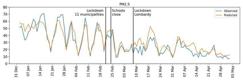
which yield qualitatively similar results, to the Supplementary information. To our knowledge,

there is little guidance in the literature on how to properly estimate standard errors in this context.

Thus, where reasonable, we cluster standard errors by monitor; where the number of clusters is

small, we use robust heteroskedasticity-standard errors.

3.1    Accuracy of predictions

To assess the accuracy of predictions, we test the counterfactual against observed values during the

pre-lockdown period from January 1 to February 22, which has not been used for training. Table

1 reports mean values of Pearson’s correlation coefficient (Corr), mean bias (MB), normalized

mean bias (nMB), and root mean square error (RMSE). As we ultimately compute the difference-

in-differences between observed values and the counterfactual, we also report the centered RMSE

(cRMSE) and the normalized centered RMSE (ncRMSE).4 For completeness, the table also includes

statistics for the training set.

   The correlation between observed and predicted values in the pre-lockdown period is 0.87 and

0.88 for PM2.5 and NO2 , respectively. The counterfactual overestimates observed values by 1.34

µg/m3 (PM2.5 ) and 4.7 µg/m3 (NO2 ), thus motivating the use of a difference-in-differences strategy.

The centered RMSE is 30% (PM2.5 ) and 27% (NO2 ) of mean observed concentrations. A graph-

ical summary of model predictive performance, Taylor diagrams, can be found in Supplementary

information.

   In air pollution forecasting, machine learning techniques are typically used to predict concen-

trations an hour to few days ahead, and studies that can be used as benchmark are scarce. To

the best of our knowledge, Petetin et al. (2020) is the only work whose methodology and length of

forecast are comparable. They use machine learning to build a counterfactual for NO2 concentra-

tions in Spain during the COVID-19 lockdown. They report a normalized mean bias of 2% to 7%,

depending on the type of station, a correlation coefficient of 0.71 to 0.75, and normalized RMSE

of 28% to 32%. Compared to their study, our algorithm better mimics variation around the mean,

                                                  8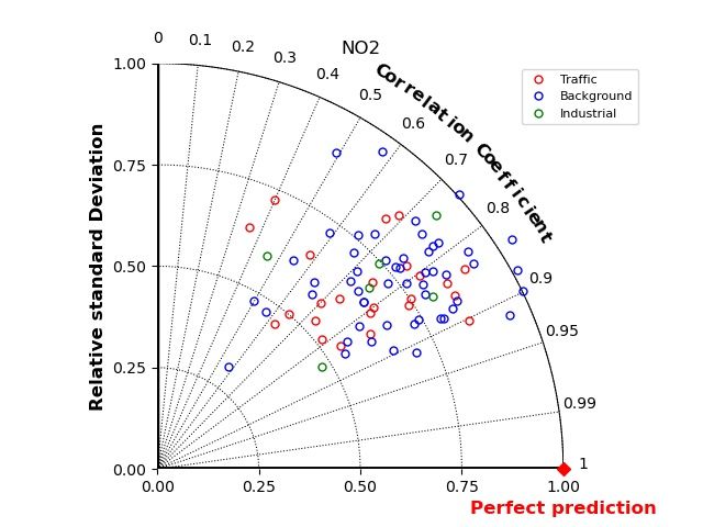
Table 1: Accuracy of predictions, average values across monitors

               Pollutant   Dataset     Corr        MB          nMB      RMSE      cRMSE   ncRMSE

               NO2         Train         1         .004          0        .276     .275    .008
               NO2         Test        .875       -4.672       -.159     9.961    8.088    .261
               PM2.5       Train       .999          0           0        .443     .443    .015
               PM2.5       Test        .871       -1.335       -.049     8.764    8.476    .295

Notes: Corr: Pearson’s correlation coefficient. MB: Mean bias, where negative values indicate observed values
below predicted values. nMB: Normalized mean bias. RMSE: Root mean squared error. nRMSE: Normalized
RMSE. cRMSE: Centered RMSE. ncRMSE: Normalized centered RMSE. Mean bias, RMSE and centered RMSE
are expressed in µg/m3 . Mean bias, RMSE and centered RMSE are normalized dividing by mean observed
                                                                              1/2
concentrations. The centered RMSE is computed as 1/N (ybi − y¯

                                                                b − yi + ȳ)2
                                                        P
                                                                                   .

than the mean itself. However, in our estimation strategy, any constant bias is captured by the

constant in Equation 1.

                                                                       1/2
                                               (ybi − y¯
  4

                                                       b − yi + ȳ)2
                                              P
      The centered RMSE is computed as 1/N                                    .

                                                           9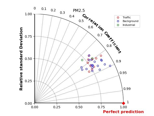
3.2       Years of life saved

To compute the number of avoided deaths and years of life saved by the reduction in PM2.5, we

follow Fowlie et al. (2019) and take all-cause mortality relative risk (RR) ratios for PM2.5 from two

influential studies, Krewski et al. (2009) and Lepeule et al. (2012). In addition, we use the RR ratio

recommended by the WHO (Henschel et al. (2013)) and adopted by the European Environment

Agency (European Environment Agency 2019). For NO2 , we only use the WHO recommendations.

        The more conservative estimates are based on Krewski et al. (2009), who report an hazard

ratio 1.056 for an increase of 10 µg/m3 of PM2.5 . Lepeule et al. (2012) estimate instead a larger

hazard ratio of 1.14 for the same change in concentrations. The WHO recommends estimating the

long-term impact of exposure to PM2.5 in adult populations using an RR of 1.062 for 10 µg/m3 ; it

recommends an RR of 1.055 for 10 µg/m3 of NO2 above 20 µg/m3 in adult populations.

4        Data

We assemble a dataset of air pollution, atmospheric conditions and calendar variables for the period

2012 to 2020 for the Italian region of Lombardy. The region is the home to about 10 million people

and is the first contributor to the national GDP by size. Its natural geography is conducive to

low winds and stable air masses throughout the cold season. Mountain ranges to the North, West

and South effectively block transboundary air streams extending wintertime thermal inversions and

aggravating pollution events. For exceeding recommended air quality thresholds, Italy has been

fined and subject to infringement procedures by the EU. We describe the data sources and pollution

trends in Lombardy.

4.1       Air pollution

Data for air pollution is collected, checked, and published by ARPA Lombardia, the regional envi-

ronmental agency.5 We obtain readings for PM2.5 and NO2 , for background, traffic, and industrial

stations as available. Hourly readings are averaged to daily readings. We exclude all monitoring
    5
    Both air pollution and weather data are publicly available at https://www.dati.lombardia.it/stories/s/
auv9-c2sj.

                                                   10
stations that are not functioning during the lockdown or have been set up after 2015. Background
stations account for about 60% of pollution monitors, traffic stations for about 30%, and the re-
maining 10% is located in industrial areas.
Average yearly concentrations of PM2.5 in Milan, the region’s capital, are systematically above
the safety levels established by the WHO (10 µg/m3 ); from December to the end of February, daily
concentrations average above 40 µg/m3 . Average levels of NO2 during the period are also well
above WHO safety standards.
4.2 Weather data
Data on weather conditions at weather stations throughout the region are also elaborated and made
available by ARPA Lombardia. We retrieve the daily minimum and maximum temperature; average
wind speed and wind direction; average relative humidity; and daily cumulative precipitation. We
further include a host of atmospheric sounding indices measured at Milano Linate airport and made
available by the University of Wyoming, namely Showalter index, Lifted index, SWEAT index, K
index, and Cross Totals, and Vertical Totals indices. All atmospheric variables enter as predictors in
the form of contemporaneous and lagged values. Although monitor data and atmospheric soundings
have gone through quality checks at the source, we winsorize all atmospheric predictors at 1 and
99 percentiles to bound the influence of extreme values.
4.3 Additional predictors
The ratio of PM2.5 to PM10 in Lombardy is typically altered in presence of pollution transported
from long distances. For instance, a mass of dust from the Caspian Sea reached Northern Italy in
late March, substantially altering the ratio. We take the PM2.5 to PM10 ratio as exogenous to the
effects of the lockdown and include it among predictors as the concentration of PM2.5 is affected
by such idiosyncratic shocks. Additional predictors are calendar variables to capture trends over
time and seasons. We include year, month, week of the year, day of the month, day of the week in
the form of continuous variables as well as dummy variables. We further include sine functions of
time to mimic seasonality.
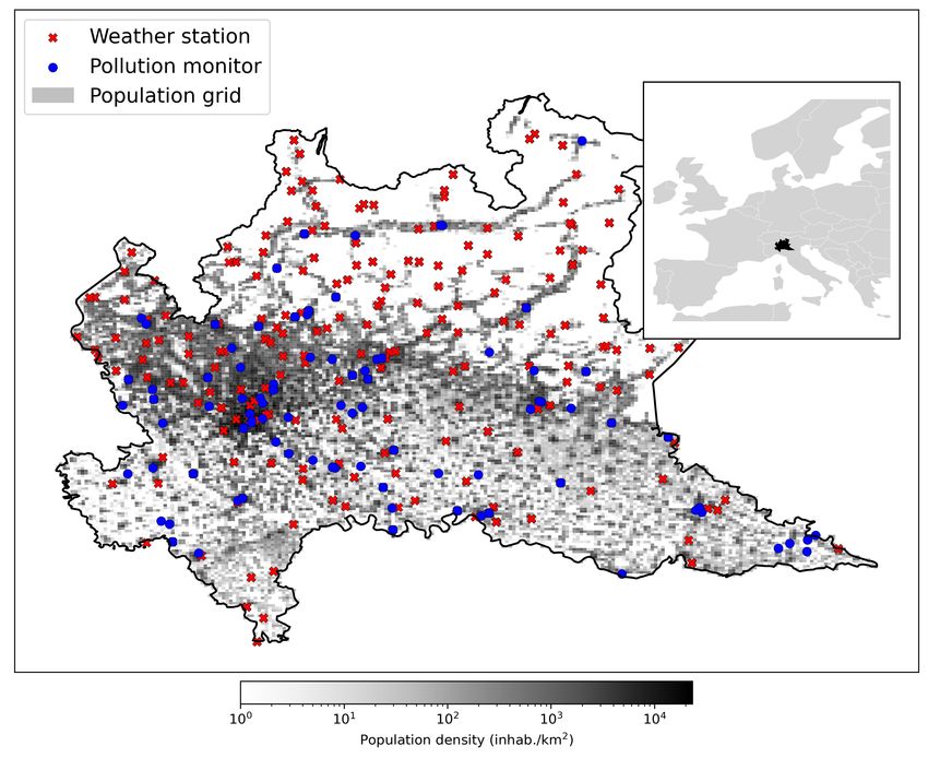
114.4 Population weights
Population weights for monitoring stations reflect the population within 20 kilometers of monitors
(Figure 3 in Supplementary information). Population data on a 1 km by 1 km grid comes from the
Italian National Statistical Office (ISTAT).6 Grid cells within less than 20 kilometers from two or
more monitors are assigned to the closest one.
5 Results and Discussion
5.1 Effect of the lockdown on air pollution
Following the lockdown, air quality in Lombardy improved substantially, albeit partially. Figure 2
plots the population-weighted observed and counterfactual values for PM2.5 (Figure 2a) and NO2
(Figure 2b). The counterfactual well mimics observed values in the pre-lockdown period, supporting
the validity of the counterfactual. In comparison, a gap between observed and counterfactual values
is evident as restrictions are tightened. We show in Supplementary information that the method
outperforms a linear regression.
Suggestive evidence of the effect of the lockdown on concentrations of NO2 , which in Lombardy
largely originate from motor vehicles, is visible from the week of February 25, consistent with the
reduction in mobility documented in Figure 1a. The effect on PM2.5 only appears as non-essential
economic activities are halted in Lombardy and the rest of Italy, and is smaller in magnitude.
6
The data is available at https://www.istat.it/it/files//2015/04/GEOSTAT_grid_POP_1K_IT_
2011-22-10-2018.zip. Last accessed on July 23, 2020.
12(a)
(b)
Figure 2: Population-weighted average of observed and counterfactual values. a, PM2.5 .
b, NO2 . Population is measured within 20 kilometers of a monitoring station. Territory within less
than 20 kilometers from two or more monitors is assigned to the closest one.
We estimate a population-weighted version of Equation 1 in Methods and report results in Table
3. Results of unweighted regressions are qualitatively similar and can be found in Supplementary
information. From February 22 to May 4, the lockdown has on average reduced daily concentrations
of PM2.5 and NO2 by 5.32 µg/m3 and 13.56 µg/m3 . That is a reduction of 21.8% and 35.6%,
respectively, from the average levels that would have been observed had not the epidemic broken
out.
Next, our preferred specification distinguishes treatment effects by type of monitor. Background
monitors are located where concentrations are representative of the ambient exposure of the general
13population; industrial monitors are located in the proximity of industrial sites or industrial sources;
traffic monitors are located near a single major road.
Population-weighted average background concentrations of PM2.5 decreased by 3.84 µg/m3 from
24.42 µg/m3 (Table 4).7 The reduction was almost twice as large in monitored industrial sites and
near major roads. Background concentrations of NO2 dropped by 10.85 µg/m3 from 33.22 µg/m3 ,
by 10.66 µg/m3 near monitored industrial sites and by 15.85 µg/m3 more at major roads.
Table 3: Population-weighted regression
∆Observed,Counterf actual
(1) (2)
PM 2.5 NO2
Lockdown -5.32∗∗∗ -13.56∗∗∗
(1.08) (1.21)
Constant 0.73 2.59
(1.37) (1.67)
Average baseline concentration 24.39 38.14
Observations 3555 10084
Notes: Regression weighted by population within 20 kilometers of
a monitoring station. Territory within less than 20 kilometers from
two or more monitors is assigned to the closest one. The dependent
variable is the difference between the observed values and the coun-
terfactual. Lockdown is a dummy variable equal to 0 from January 1,
2020 to February 22, and equal to 1 after February 22, 2020. Average
baseline concentration is the population-weighted average of coun-
terfactual values during the lockdown, less the constant in case the
latter is statistically significant at 10%. Standard errors, in brackets,
are clustered by monitor. * pTable 4: Heterogeneous effects by type of monitoring station
∆Observed,Counterf actual
PM 2.5 NO2
Background Industrial Traffic Background Industrial Traffic
Lockdown -3.84∗∗∗ -7.39∗∗∗ -7.28∗∗∗ -10.85∗∗∗ -10.66∗∗∗ -15.85∗∗∗
(0.97) (1.54) (1.20) (0.64) (0.96) (0.75)
Constant -1.26 5.18∗∗∗ 2.79∗∗ 0.21 7.29∗∗∗ 4.04∗∗∗
(0.84) (1.37) (1.07) (0.49) (0.84) (0.63)
Average baseline concentration 24.42 27.99 27.77 33.22 31.93 46.67
Number of monitors 18 2 10 53 6 24
Observations 2117 244 1194 6483 731 2870
Notes: Regression weighted by population within 20 kilometers of a monitoring station. Territory within less than 20 kilometers
from two or more monitors is assigned to the closest one. The dependent variable is the difference between the observed values and
the counterfactual. Lockdown is a dummy variable equal to 0 from January 1, 2020 to February 22, and equal to 1 after February
22, 2020. Average baseline concentration is the population-weighted average of counterfactual values during the lockdown, less
the constant in case the latter is statistically significant at 10%. Robust standard errors are in brackets. * p5.2 Human health benefits
As the reduction in road transport and the slowing of economic activity reduced toxic emissions, the
burden of pollutants on human health eased. We compute avoided deaths and the years of life that
have been saved (YLS) by the improvement in air quality following the recommendations of the
WHO (Henschel et al. 2013) and the methodology of the European Environment Agency (European
Environment Agency 2019). We also follow Fowlie et al. (2019) and adopt concentration-response
functions for PM2.5 from two influential studies for lower- and upper-bound estimates (Krewski
et al. 2009; Lepeule et al. 2012).8 For calculations, we use the estimated change in concentrations
at background stations.
The reduction in PM2.5 prevented 10.2 to 24.8 premature deaths per 100,000 individuals and
saved 72.1 to 175.9 years of life per 100,000 individuals, depending on the concentration-response
function (Table 5). The reduction in NO2 prevented 28.8 premature deaths and saved 203.7 years of
life per 100,000 individuals. Given the high correlation between concentrations of PM2.5 and NO2 ,
the concentration-response function of these pollutants are interdependent. It is recommended
that avoided deaths and YLS be not aggregated across pollutants, lest incurring in partial double
counting.
As a comparison, in Italy in 2016 for every 100,000 individuals, there have been 96.6 premature
deaths attributable to PM2.5 and 24.1 attributable to NO2 , or 23.8 and 5.9 premature deaths
in three months, respectively (European Environment Agency 2019). Since most of the prema-
ture deaths happen in the more polluted North of Italy, including Lombardy, the lockdown has
temporarily reduced the cost of pollution by a substantial amount.
To appreciate the magnitude of avoided deaths and YLS, we compare it against the number of
deaths related to COVID-19 and the years of life lost (YLL) in Lombardy during the same period,
computed from patient-level data.9 In Lombardy, from February 22 to May 3 2020, every 100,000
people 155 died after testing positive for COVID-19 and 1891 years of life have been directly lost
to the virus. Avoided deaths from the reduction in PM2.5 are 6.5% to 16% of COVID-19 deaths;
16Table 5: Avoided premature deaths and years of life saved per 100,000 in Lombardy due to improved
air quality during lockdown.
Pollutant Source of HR Hazard ratio Avoided deaths
Avoided deaths NO2 EEA/WHO 1.055 28.8
PM 2.5 EEA/WHO 1.062 11.3
PM 2.5 Krewski et al. (2009) 1.056 10.2
PM 2.5 Lepeule et al. (2012) 1.14 24.8
Years of life saved NO2 EEA/WHO 1.055 203.7
PM 2.5 EEA/WHO 1.062 79.7
PM 2.5 Krewski et al. (2009) 1.056 72.1
PM 2.5 Lepeule et al. (2012) 1.14 175.9
In Lombardy, from February 22 to May 3 2020, every 100,000 people 155 died after testing positive for COVID-19
and 1891 years of life have been directly lost to the virus. The hazard ratio is the ratio of two concentration-response
functions, or hazard rates, between a high and a low concentration differing by 10 µg/m3 . Avoided premature
deaths are calculated using the population-weighted change in concentrations at background stations.
YLS are 3.8% to 9.3% of YLL to COVID-19. Avoided deaths from the reduction in NO2 are 18.6%
of COVID-19 deaths; YLS are 10.8% of YLL to COVID-19.
8
See Supplemetary Material for more details.
9
Data on the individual COVID-19 patients has been shared by regional health officers under an institutional
agreement.
176 Conclusions
The dramatic reduction in emissions of airborne pollutants that has come with the response to
COVID-19 provides a unique natural experiment to assess the sensitivity of concentrations of pol-
lutants to emissions. We estimate a substantial yet partial improvement in air quality in Lombardy
following the outbreak, and suggest that the improvement originates primarily from the reduc-
tion of road transport; and to a lesser degree from the reduction in industrial activity. Important
sources of emissions as heating systems and agriculture have not been substantially affected by the
outbreak; as a consequence, the improvement in air quality has been partial.
We estimate the effect of a temporally well-defined reduction in emissions on concentrations.
The methodology used to build the counterfactual does not require identifying comparable but
unaffected units, but relies on the assumption of emissions following historical variation around
the mean absent the lockdown. This approach can be applied in a variety of settings due to the
increasing and reliable availability of pollution and weather data.
Finally, we are nowhere near suggesting the pandemic has been beneficial for the affected com-
munities, yet the health benefits from improved air quality are noticeable. While global pandemics
are rare phenomena, exposure to unhealthy levels of toxic air pollutants is the rule, including in
affluent parts of the world such as the one considered here. This paper has emphasized the health
benefits of cleaner air, but also highlighted the variety of emissions sources and the need for a
broader policy response to solve Europe’s biggest environmental health risk.
References
Amini, H., Nhung, N. T. T., Schindler, C., Yunesian, M., Hosseini, V., Shamsipour, M., Hassan-
vand, M. S., Mohammadi, Y., Farzadfar, F., Vicedo-Cabrera, A. M., et al. (2019). Short-term
associations between daily mortality and ambient particulate matter, nitrogen dioxide, and the
air quality index in a middle eastern megacity. Environmental Pollution, 254:113121.
Apple (2020). COVID-19 Mobility Trends Reports. Data retrieved from https://www.apple.com/
covid19/mobility. Last accessed on September 22, 2020.
18Chen, T. and Guestrin, C. (2016). XGBoost: A Scalable Tree Boosting System. In Proceedings
of the 22nd ACM SIGKDD International Conference on Knowledge Discovery and Data Mining,
pages 785–794.
Cole, M. A., Elliott, R. J. R., and Liu, B. (2020). The Impact of the Wuhan Covid-19 Lockdown
on Air Pollution and Health: A Machine Learning and Augmented Synthetic Control Approach.
Environmental and Resource Economics, 76(4):553–580.
Deryugina, T., Heutel, G., Miller, N. H., Molitor, D., and Reif, J. (2019). The Mortality and
Medical Costs of Air Pollution: Evidence from Changes in Wind Direction. American Economic
Review, 109(12):4178–4219.
Duan, Y., Liao, Y., Li, H., Yan, S., Zhao, Z., Yu, S., Fu, Y., Wang, Z., Yin, P., Cheng, J., et al.
(2019). Effect of changes in season and temperature on cardiovascular mortality associated with
nitrogen dioxide air pollution in Shenzhen, China. Science of The Total Environment, 697:134051.
Ebenstein, A., Fan, M., Greenstone, M., He, G., and Zhou, M. (2017). New evidence on the
impact of sustained exposure to air pollution on life expectancy from China’s Huai River Policy.
Proceedings of the National Academy of Sciences, 114(39):10384–10389.
Ebenstein, A., Lavy, V., and Roth, S. (2016). The long-run economic consequences of high-stakes
examinations: Evidence from transitory variation in pollution. American Economic Journal:
Applied Economics, 8(4):36–65.
European Environment Agency (2019). Air quality in Europe - 2019 report.
Fowlie, M., Rubin, E., and Walker, R. (2019). Bringing satellite-based air quality estimates down
to earth. AEA Papers and Proceedings, 109:283–88.
Friedman, J. H. (2001). Greedy function approximation: a gradient boosting machine. Annals of
statistics, pages 1189–1232.
Google (2020). COVID-19 Community Mobility Reports. Data retrieved from https://www.
google.com/covid19/mobility/. Last accessed on June 27, 2020.
19Graff Zivin, J. and Neidell, M. (2012). The Impact of Pollution on Worker Productivity. American
Economic Review, 102(7):3652–3673.
Guo, S., Hu, M., Zamora, M. L., Peng, J., Shang, D., Zheng, J., Du, Z., Wu, Z., Shao, M., Zeng,
L., Molina, M. J., and Zhang, R. (2014). Elucidating severe urban haze formation in China.
Proceedings of the National Academy of Sciences, 111(49):17373–17378.
He, G., Pan, Y., and Tanaka, T. (2020). The short-term impacts of COVID-19 lockdown on urban
air pollution in China. Nature Sustainability.
He, J., Liu, H., and Salvo, A. (2019). Severe Air Pollution and Labor Productivity: Evidence from
Industrial Towns in China. American Economic Journal: Applied Economics, 11(1):173–201.
Henschel, S., Chan, G., Organization, W. H., et al. (2013). Health risks of air pollution in europe-
hrapie project: New emerging risks to health from air pollution-results from the survey of experts.
INEMAR (2017). INEMAR - Inventario Emissioni Aria. Last accessed on June 15, 2020. Data
retrieved from http://inemar.arpalombardia.it/inemar/webdata/main.seam?cid=22157.
Kahn, M. E. and Li, P. (2020). Air pollution lowers high skill public sector worker productivity in
China. Environmental Research Letters, 15(8):084003.
Krewski, D., Jerrett, M., Burnett, R. T., Ma, R., Hughes, E., Shi, Y., Turner, M. C., Pope III,
C. A., Thurston, G., Calle, E. E., et al. (2009). Extended follow-up and spatial analysis of the
American Cancer Society study linking particulate air pollution and mortality. Number 140.
Health Effects Institute Boston, MA.
Kroll, J. H., Heald, C. L., Cappa, C. D., Farmer, D. K., Fry, J. L., Murphy, J. G., and Steiner, A. L.
(2020). The complex chemical effects of COVID-19 shutdowns on air quality. Nature Chemistry,
12(9):777–779.
Lepeule, J., Laden, F., Dockery, D., and Schwartz, J. (2012). Chronic exposure to fine parti-
cles and mortality: an extended follow-up of the Harvard Six Cities study from 1974 to 2009.
Environmental health perspectives, 120(7):965–970.
20Mills, I. C., Atkinson, R. W., Kang, S., Walton, H., and Anderson, H. (2015). Quantitative system-
atic review of the associations between short-term exposure to nitrogen dioxide and mortality
and hospital admissions. BMJ open, 5(5).
Petetin, H., Bowdalo, D., Soret, A., Guevara, M., Jorba, O., Serradell, K., and Pérez García-Pando,
C. (2020). Meteorology-normalized impact of COVID-19 lockdown upon NO2 pollution in Spain.
Atmospheric Chemistry and Physics Discussions, 2020:1–29.
Pope, C. A. I. and Dockery, D. W. (2006). Health Effects of Fine Particulate Air Pollution: Lines
that Connect. Journal of the Air & Waste Management Association, 56(6):709–742.
Silver, B., He, X., Arnold, S. R., and Spracklen, D. V. (2020). The impact of COVID-19 control
measures on air quality in china. Environmental Research Letters, 15(8):084021.
TERNA (2020). Transparency Report. Data retrieved from https://www.terna.it/it/
sistema-elettrico/transparency-report/download-center. Last accessed on June 28, 2020.
Zhang, X., Chen, X., and Zhang, X. (2018). The impact of exposure to air pollution on cognitive
performance. Proceedings of the National Academy of Sciences, 115(37):9193–9197.
21A Supplementary information
A.1 Years of life saved
Concentration-response functions are typically estimated with log-linear regressions of mortality
risk on pollutants of the form ln(y) = α + βC, so that y = AeβC . The change in mortality risk
from y 0 to y 00 is
0 00
y 0 − y 00 = A(eβC − eβC )
0 00 −C 0 )
= AeβC (1 − eβ(C )
1
= y 0 (1 − )
eβ(C 0 −C 00 )
0 00 )
with A = eα . Here y 0 is the baseline mortality risk and eβ(C −C is the RR. The β coefficient is
not typically reported, but is easily found as β = ln(RR)/10.
For each gender g and age group a above 30, we multiply the change in mortality risk from the
baseline by the number of individuals in Lombardy of that gender and age group (Ng,a ).10 This
gives us the number of avoided deaths for a year-long reduction in pollutants. We then multiply
this number by gender- and age-specific life expectancy to obtain the YLS.
0 1
Avoided Deathsg,a = yg,a · (1 − ) · Ng,a
eβ(C 0 −C 00 )
1
Y LSg,a = Avoided Deathsg,a · Lif e Expectancyg,a ·
6
XX
Y LS = Y LSg,a
g a
It should be noted that we are assuming that avoided deaths and years of life saved by a
two-month improvement in air quality are equivalent to a sixth of the benefits of a year-long
improvement. In addition, we assume that the gains are linear in reductions of concentrations.11
Gender- and age-group specific baseline mortality risk, population size and life expectancy come
from mortality tables for Lombardy compiled by the Italian National Statistical Office (ISTAT).
10
The benefits from reductions in NO2 are set to zero for values below 20 µg/m3 , as recommended by Henschel
et al. (2013).
11
This is in line with Henschel et al. (2013), who recommend a linear concentrations-response function.
22Avoided deaths and YLS are computed using the lockdown on pollution (C 0 − C 00 ) estimated at
background stations.
A.2 Accuracy of linear regression for construction of counterfactuals
We show a linear regression model does not perform as well as the machine learning algorithm
used for the main results. For every monitoring station, we regress daily concentrations on a
vector of daily weather summaries, namely daily cumulative precipitation, average temperature,
average wind speed and average wind direction, in 2012 through 2019 (Equation 2). We then use
the estimated coefficients to predict concentrations in 2020 before and throughout the lockdown
(Equation 3). Finally, we assess the accuracy of predictions during the pre-lockdown period from
January 1 to February 21, 2020. Precipitation, temperature, wind speed and direction on day t
at any given pollution monitor are interpolated with inverse distance weight from the three closest
weather stations within 0.2 degrees from the monitor.
yt2012−2019 = α + β 0 W eathert2012−2019 + t2012−2019 (2)
b + βb0 W eathert2020
ybt2020 = α (3)
Observed and predicted population-weighted average concentrations are displayed in Figure 3.
While approximating pre-lockdown values on average, the predictions fail to capture a non-negligible
portion of the variability. The validity of predictions based on linear regressions is especially poor
for PM2.5 . The same conclusions can be drawn examining average accuracy measures for linear
regression predictions in Table 7.
23Table 7: Accuracy of liner regression predictions, average values across monitors
Pollutant Dataset Corr MB nMB RMSE cRMSE ncRMSE
NO2 Train 0.71 0 0 9.7 9.7 0.33
NO2 Test 0.7 -5.09 -0.16 13.22 11.45 0.37
PM2.5 Train 0.63 0 0 12.21 12.21 0.53
PM2.5 Test 0.59 0.35 0.01 14.43 14.21 0.5
Notes: Corr: Pearson’s correlation coefficient. MB: Mean bias, where negative values indicate observed values
below predicted values. nMB: Normalized mean bias. RMSE: Root mean squared error. nRMSE: Normalized
RMSE. cRMSE: Centered RMSE. ncRMSE: Normalized centered RMSE. Mean bias, RMSE and centered RMSE
are expressed in µg/m3 . Mean bias, RMSE and centered RMSE are normalized dividing by mean observed
1/2
(ybi − y¯
b − yi + ȳ)2
P
concentrations. The centered RMSE is computed as 1/N .
24(a)
(b)
Figure 3: Population-weighted average of observed and counterfactual values built with
linear regression models. a, PM2.5 . b, NO2 . Population is measured within 20 kilometers of a
monitoring station. Territory within less than 20 kilometers from two or more monitors is assigned
to the closest one.
25A.3 Supplementary tables
Table 8: Pollution monitors by type.
Pollutant Type of monitor Number of municipalities Number of monitors
NO2 Background 50 53
NO2 Industrial 6 6
NO2 Traffic 20 24
PM2.5 Background 18 18
PM2.5 Industrial 2 2
PM2.5 Traffic 10 10
Background stations measure pollutions concentrations that are representative of the average exposure of the
general population, or vegetation. Industrial stations are located in close proximity to an industrial area or an
industrial source. Traffic stations are located in close proximity to a single major road.
26Table 10: Unweighted regression
∆Observed,Counterf actual
(1) (2)
PM 2.5 NO2
Lockdown -4.37∗∗∗ -9.19∗∗∗
(0.41) (0.65)
Constant 1.19∗∗ 0.73
(0.47) (0.53)
Average baseline concentration 25.58 38.14
Observations 3555 10084
Notes: Unweighted regression. The dependent variable is the differ-
ence between the observed values and the counterfactual. Lockdown
is a dummy variable equal to 0 from January 1, 2020 to February
22, and equal to 1 after February 22, 2020. Average baseline concen-
tration is the average of counterfactual values during the lockdown,
less the constant in case the latter is statistically significant at 10%.
Standard errors, in brackets, are clustered by monitor. * pTable 11: Heterogeneous effects by type of monitoring station - unweighted regression
∆Observed,Counterf actual
PM 2.5 NO2
Background Industrial Traffic Background Industrial Traffic
Lockdown -3.70∗∗∗ -7.63∗∗∗ -4.92∗∗∗ -7.53∗∗∗ -7.50∗∗∗ -13.39∗∗∗
(0.39) (1.33) (0.53) (0.19) (0.58) (0.39)
Constant 0.79∗ 5.10∗∗∗ 1.11∗ -0.05 2.89∗∗∗ 1.98∗∗∗
(0.34) (1.20) (0.46) (0.15) (0.48) (0.31)
Average baseline concentration 25.21 27.91 26.09 33.22 27.53 44.61
Number of monitors 18 2 10 53 6 24
Observations 2117 244 1194 6483 731 2870
Notes: Unweighted regression. The dependent variable is the difference between the observed values and the counterfactual.
Lockdown is a dummy variable equal to 0 from January 1, 2020 to February 22, and equal to 1 after February 22, 2020.
Average baseline concentration is the average of counterfactual values during the lockdown, less the constant in case the latter is
statistically significant at 10%. Robust standard errors are in brackets. * pA.4 Supplementary figures
Figure 4: Location of pollution monitors and weather stations in Lombardy over a 1 km by 1 km
population grid.
29(a) PM2.5
(b) NO2
Figure 5: Taylor diagrams are a practical way to display different dimensions of model predictive
performance (Taylor 2001). Each circle represents the prediction of a model, that is, in this case, a
monitoring station for the pre-lockdown period from January 1 to February 22. Isocurves from the
origin outward measure the standard deviation of a model’s predictions relative to the standard
deviation of the observed values. The azimut measures Pearson’s correlation coefficient. The ideal
model prediction has a relative standard deviation of 1 and a correlation coefficient of 1, and is
marked by the red diamond. We do not show the RMSE, as is practice in Taylor diagrams, because
it is graphically incompatible with the relative standard
30 deviation.Figure 6: Each polygon circumscribes the territory nearest to a monitor and within 20 kilometers
from it. Color represents population in grid cells of 1 km2 .
31A.5 Lockdown of Lombardy
Italy has witnessed one of the first major outbreak of COVID-19 outside China. The virus has
first been identified in two Chinese tourists who had arrived at Milano Malpensa Airport and, on
January 31st, tested positive for the virus when visiting Rome (ANSA 2020b). For the next three
weeks, only a handful of cases had been identified and all had a direct link with known hot-spots,
such as a student returning from vacation in Wuhan and a couple of tourists from Taiwan (ANSA
2020a,c).
However, on February 21st, the first non-imported cases and the first death related to COVID-
19 in the country were confirmed in lower Lombardy. By the end of the day, 17 individuals had
been tested positive, 15 of which in Lodi and surroundings, in lower Lombardia, and 2 in the
neighboring region of Veneto. The largest hotspot had been identified in the hospital of Codogno,
where 5 members of the medical staff and 3 patients had tested positive to COVID-19. On the
same day, the Minister of Health announced severely restrictive measures on 11 municipalities
and over 50 000 people. Until further notice, schools and all public and sporting events were
suspended; non-essential production, commercial activities and public offices had to close doors;
self-isolation at home was mandated and enforced; access to the municipalities was monitored by
police and armed forces (Presidente del Consiglio dei Ministri 2020c; ANSA 2020d; La Repubblica
2020; Guidelli 2020) Also, self-isolation for two weeks was mandatory for whoever in the country
had had contacts with confirmed cases. Violations of lockdown areas and self-isolation could be
sanctioned with fines and up to a three months prison sentence (Presidente della Repubblica 2020;
Ministro della Salute 2020a).
Over the next two days, local governments all over the country imposed restrictions of hetero-
geneous degrees, with strictest measures in the regions of Lombardia and Veneto. In Lombardia,
the regional government suspended all teaching activities in schools and universities, prohibited
public events, and suspended religious gatherings; pubs had to close by 6 pm (Ministro della Salute
2020b).
Local measures were soon followed by the intervention of the central government. On February
25th, the Prime Minister signed a Law Degree to expand and incorporate containment efforts in
32hotspot regions of Northern Italy. The decree closed schools and universities (originally until March
15th) and recommended remote working in Emilia Romagna, Friuli Venezia Giulia, Lombardia,
Veneto, Liguria, and Piemonte (Presidente del Consiglio dei Ministri 2020d).
A week later, on March 1st, the government extends previous measures and prescribes non-
restrictive ones over non-affected regions(Presidente del Consiglio dei Ministri 2020b); on March
4th, it announces all schools and universities in the countries will close.
By March 7th, 5883 cases had been confirmed in Italy and 233 COVID-19-related deaths
recorded (Protezione Civile 2020). Despite containment measures, the growing number of con-
firmed cases and deaths pressured the Italian government to impose stricter controls. With a Law
Decree on March 8th, Italy became the first country in Europe to impose a lockdown over Lombar-
dia and 14 provinces of the northern and central regions of Piemonte, Emilia-Romagna, Veneto, and
Marche. The restrictive measures were soon extended to the rest of the country on the following
day. The decree imposed compulsory social distancing and self-isolation at home and the halt of
all non-essential economic activities (Presidente del Consiglio dei Ministri 2020a; Presidenza del
Consiglio dei Ministri 2020).
The list of sectors and activities deemed essential had been furthered narrowed on March 23rd;
most notably, construction works were stopped, and all public offices had to close (Presidente del
Consiglio dei Ministri 2020e). The lockdown then continued under virtually unaltered conditions
until May 3rd.
References in Supplementary information
[SI1] ANSA (2020a). Coronavirus: contagiato è reggiano, era in Cina in vacanza. https://www.ansa.
it/emiliaromagna/notizie/2020/02/07/coronavirusitaliano-in-buone-condizioni_
a8e7dccc-ad92-4fe7-ad06-6e5d00d9c57a.html. Last accessed on July 28, 2020.
[SI2] ANSA (2020b). Coronavirus: coppia Taiwan in Toscana dal 26
al 29 gennaio. https://www.ansa.it/toscana/notizie/2020/02/
3309/coronavirus-coppia-taiwan-in-toscana-dal-26-al-29-febbraio_
99d50b7f-62fc-4822-ba9d-cbc9e447ebe1.html. Last accessed on July 28, 2020.
[SI3] ANSA (2020c). Coronavirus: coppia Taiwan in Toscana dal 26
al 29 gennaio. https://www.ansa.it/toscana/notizie/2020/02/
09/coronavirus-coppia-taiwan-in-toscana-dal-26-al-29-febbraio_
99d50b7f-62fc-4822-ba9d-cbc9e447ebe1.html. Last accessed on July 28, 2020.
[SI4] ANSA (2020d). Coronavirus, sedici nuovi contagiati. Due sono in Veneto.
Altri 8 casi a Codogno, 5 operatori sanitari. https://www.ansa.it/
lombardia/notizie/2020/02/21/coronavirus-sedici-nuovi-contagiati.
-due-sono-in-veneto.-altri-8-casi-a-codogno-5-operatori-sanitari_
c7a81b85-4370-46b8-a2db-9a7a4df05d90.html. Last accessed on July 28, 2020.
[SI5] Guidelli, M. (2020). Coronavirus in Italia: scattato l’isolamento dei focolai, 43
varchi e 500 uomini. ANSA.it. https://www.ansa.it/canale_saluteebenessere/
notizie/sanita/2020/02/23/coronavirus-in-italia-aumentano-i-contagi.
-scuole-chiuse-in-lombardia-e-veneto.-stop-al-carnevale-di-venezia_
40e888b6-8418-406a-9771-7a6c3c0b45fd.html. Last accessed on July 28, 2020.
[SI6] La Repubblica (2020). Coronavirus, in dieci comuni lombardi: 50 mila persone costrette a
restare in casa. Quarantena all’ospedale milanese di Baggio. https://milano.repubblica.
it/cronaca/2020/02/21/news/coronavirus_codogno_castiglione_d_adda_contagiati_
misure_sicurezza-249154447/. Last accessed on July 28, 2020.
[SI7] Ministro della Salute (2020a). Ordinanza 21 febbraio 2020 Ulteriori misure profilattiche contro la
diffusione della malattia infettiva COVID-19. (20A01220) . Gazzetta Ufficiale Serie Generale n.44
del 22-02-2020.
[SI8] Ministro della Salute (2020b). Ordinanza 23 febbraio 2020 Misure urgenti in materia di conteni-
mento e gestione dell’emergenza epidemiologica da COVID-19. Regione Lombardia. (20A01273).
Gazzetta Ufficiale Serie Generale n.47 del 25-02-2020.
34[SI9] Presidente del Consiglio dei Ministri (2020a). Decreto del Presidente del Consiglio dei Ministri
8 marzo 2020 Ulteriori disposizioni attuative del decreto-legge 23 febbraio 2020, n. 6, recante
misure urgenti in materia di contenimento e gestione dell’emergenza epidemiologica da COVID-
19. (20A01522). Gazzetta Ufficiale Serie Generale n.59 del 08-03-2020.
[SI10] Presidente del Consiglio dei Ministri (2020b). Decreto del Presidente del Consiglio dei Ministri
1 marzo 2020 Ulteriori disposizioni attuative del decreto-legge 23 febbraio 2020, n. 6, recante
misure urgenti in materia di contenimento e gestione dell’emergenza epidemiologica da COVID-
19. (20A01381). Gazzetta Ufficiale Serie Generale n.52 del 01-03-2020.
[SI11] Presidente del Consiglio dei Ministri (2020c). Decreto del Presidente del Consiglio dei Ministri 25
febbraio 2010. Ulteriori disposizioni attuative del decreto-legge 23 febbraio 2020, n. 6, recante
misure urgenti in materia di contenimento e gestione dell’emergenza epidemiologica da COVID-
19. Gazzetta Ufficiale Serie Generale n.47 del 25-02-2020.
[SI12] Presidente del Consiglio dei Ministri (2020d). Decreto del Presidente del Consiglio dei Ministri
25 febbraio 2020 Ulteriori disposizioni attuative del decreto-legge 23 febbraio 2020, n. 6, recante
misure urgenti in materia di contenimento e gestione dell’emergenza epidemiologica da COVID-
19. (20A01278). Gazzetta Ufficiale Serie Generale n.47 del 25-02-2020.
[SI13] Presidente del Consiglio dei Ministri (2020e). Decreto del Presidente del Consiglio dei Minsitri
22 marzo 2020 Ulteriori disposizioni attuative del decreto-legge 23 febbraio 2020, n. 6, recante
misure urgenti in materia di contenimento e gestione dell’emergenza epidemiologica da COVID-
19, applicabili sull’intero territorio nazionale. (20A01807). Gazzetta Ufficiale Serie Generale n.76
del 22-03-2020.
[SI14] Presidente della Repubblica (2020). Decreto-legge 23 febbraio 2020, n. 6 Misure urgenti in materia
di contenimento e gestione dell’emergenza epidemiologica da COVID-19 (20G00020). Decreto-
Legge convertito con modificazioni dalla L. 5 marzo 2020, n. 13 (in G.U. 09/03/2020, n. 61).
Gazzetta Ufficiale Serie Generale n.45 del 23-02-2020. https://www.gazzettaufficiale.it/
eli/id/2020/02/23/20G00020/sg%7D%7BGazzettaUfficiale.
35[SI15] Presidenza del Consiglio dei Ministri (2020). IoRestoaCasa, misure per il contenimento e gestione
dell’emergenza epidemiologica. http://www.governo.it/it/iorestoacasa-misure-governo.
[SI16] Protezione Civile (2020). Dati COVID-19 Italia - Public repository of the Protezione Civile. Last
accessed on July 28, 2020.
[SI17] Taylor, K. E. (2001). Summarizing multiple aspects of model performance in a single diagram.
Journal of Geophysical Research: Atmospheres, 106(D7):7183–7192.
36You can also read