Observed decreases in on-road CO2 concentrations in Beijing during COVID-19 restrictions
←
→
Page content transcription
If your browser does not render page correctly, please read the page content below
Atmos. Chem. Phys., 21, 4599–4614, 2021
https://doi.org/10.5194/acp-21-4599-2021
© Author(s) 2021. This work is distributed under
the Creative Commons Attribution 4.0 License.

Observed decreases in on-road CO2 concentrations in Beijing
during COVID-19 restrictions
Di Liu1 , Wanqi Sun2 , Ning Zeng3,4 , Pengfei Han1 , Bo Yao2 , Zhiqiang Liu1 , Pucai Wang5 , Ke Zheng1 , Han Mei1 , and
Qixiang Cai1
1 Laboratory of Numerical Modeling for Atmospheric Sciences & Geophysical Fluid Dynamics, Institute of Atmospheric
Physics, Chinese Academy of Science, Beijing, China
2 Meteorological Observation Centre, China Meteorological Administration, Beijing, China
3 Department of Atmospheric and Oceanic Science, University of Maryland, College Park, MD, USA
4 Earth System Science Interdisciplinary Center, University of Maryland, College Park, MD, USA
5 Laboratory for Middle Atmosphere and Global Environment Observation, Institute of Atmospheric Physics, Chinese

Academy of Sciences, Beijing, China

Correspondence: Pengfei Han (pfhan@mail.iap.ac.cn) and Bo Yao (yaob@cma.gov.cn)

Received: 16 September 2020 – Discussion started: 12 October 2020
Revised: 3 February 2021 – Accepted: 13 February 2021 – Published: 25 March 2021

Abstract. To prevent the spread of the COVID-19 epidemic,        LST). The enhancements during rush hours (07:00–09:00
restrictions such as “lockdowns” were conducted globally,        and 17:00–20:00 LST) were almost twice those during work-
which led to a significant reduction in fossil fuel emissions,   ing hours, indicating that emissions during rush hours were
especially in urban areas. However, CO2 concentrations in        much higher. For DC and BC, the enhancement reductions
urban areas are affected by many factors, such as weather,       during rush hours were much larger than those during work-
biological sinks and background CO2 fluctuations. Thus, it is    ing hours. Our findings showed a clear CO2 concentration
difficult to directly observe the CO2 reductions from sparse     decrease during COVID-19 restrictions, which is consistent
ground observations. Here, we focus on urban ground trans-       with the CO2 emissions reductions due to the pandemic.
portation emissions, which were dramatically affected by         The enhancement method used in this study is an effective
the restrictions, to determine the reduction signals. We con-    method to reduce the impacts of weather and background
ducted six series of on-road CO2 observations in Beijing         fluctuations. Low-cost sensors, which are inexpensive and
using mobile platforms before (BC), during (DC) and af-          convenient, could play an important role in further on-road
ter (AC) the implementation of COVID-19 restrictions. To         and other urban observations.
reduce the impacts of weather conditions and background
fluctuations, we analyze vehicle trips with the most simi-
lar weather conditions possible and calculated the enhance-
ment metric, which is the difference between the on-road         1   Introduction
CO2 concentration and the “urban background” CO2 con-
centration measured at the tower of the Institute of Atmo-       Since December 2019, the world has been fiercely strug-
spheric Physics (IAP), Chinese Academy of Sciences. The          gling with a pandemic of a novel coronavirus named COVID-
results showed that the DC CO2 enhancement was decreased         19, which was first identified in Wuhan, China (Gross et
by 41 (±1.3) parts per million (ppm) and 26 (±6.2) ppm           al., 2020), and then quickly identified in other countries
compared to those for the BC and AC trips, respectively.         of East Asia, Europe and the United States according to
Detailed analysis showed that, during COVID-19 restric-          World Health Organization Novel Coronavirus (2019-nCoV)
tions, there was no difference between weekdays and week-        situation reports (https://www.who.int/emergencies/diseases/
ends during working hours (09:00–17:00 local standard time;      novel-coronavirus-2019/situation-reports, last access: De-
                                                                 cember 2020). In Beijing, the first case was confirmed on

Published by Copernicus Publications on behalf of the European Geosciences Union.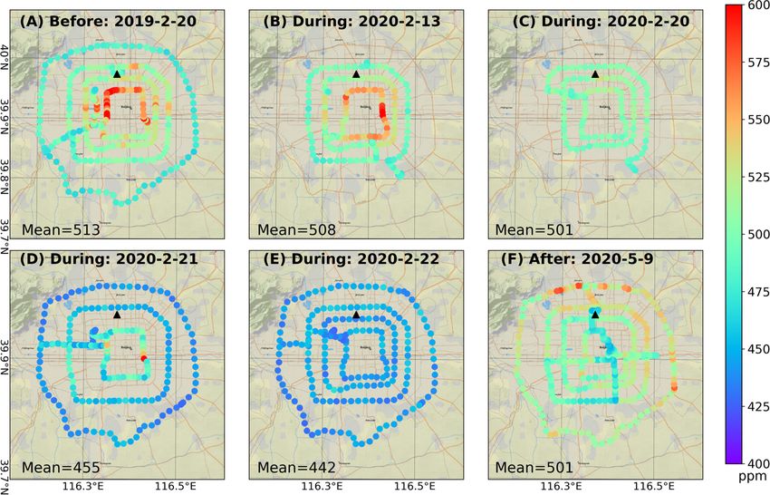
4600                                                       D. Liu et al.: Observed decreases in on-road CO2 concentrations

20 January 2020, followed by a quick increase in confirmed        ing Total Carbon Column Observation Network (TCCON)
cases (Fig. S1A). From 24 January to 30 April, Beijing en-        data. By assuming that the COVID-19-related CO2 growth
acted a level-1 response to major public health emergencies       rate reduction of 0.32 ppm yr2 in 2020 at Mauna Loa is true
(red region in Fig. S1) and lowered the response to level 2       and measured (from the UK Met Office; an overall 8 % emis-
from 30 April to 6 June, after “zero growth” persisted for        sion reduction in 2020), they found that there is a ∼ 0.6 year
almost 1 month (yellow region in Fig S1).                         “delay” to separates TCCON-measured growth rates and the
   As the world faced this highly infectious pandemic with-       reference forecast (absence of COVID-19 restrictions).
out efficient medication, governments enacted similar re-            With the knowledge that urban ground transportation was
strictions to prevent the spread of the virus: isolating cases,   strongly suppressed due to COVID-19 restrictions, we de-
enacting stay-at-home orders, forbidding mass gatherings          signed on-road observations by using a mobile platform to
and closing factories and schools. These restrictions highly      detect reduction signals. These observations could provide
altered the industrial production, energy consumption and         CO2 data with higher spatiotemporal resolution than satel-
transportation volume and led to sharp emission reductions        lite and ground observations and have been widely used for
(Liu et al., 2020; Le Quere et al., 2020). As previous in-        carbon monitoring in urban and suburban areas (for instance,
ventory studies estimated, by early April 2020, the global        on-road CO2 concentration distributions were presented as
daily CO2 emissions had decreased by 17 % (11 % to 25 %           transects in urban areas along routes) (Idso et al., 2001; Bush
for ±1σ ) compared with those in 2019, and the total reduc-       et al., 2015; Sun et al., 2019). Almost all studies agreed that
tion was approximately 1048 (543 to 1638) MtCO2 at the            weather (for example, wind speed, which is directly associ-
end of April (Le Quere et al., 2020). Emissions from ground       ated with CO2 mixing and dilution) is a dominant factor and
transportation obviously decreased by 36 % (Le Quere et al.,      should be considered during analysis. Reducing the impact
2020). According to Liu et al. (2020), emissions in China de-     of weather is still problematic. On the other hand, examin-
creased 7 % from January to April 2020, with ground trans-        ing the enhancement, which is the calculated difference in
portation emissions dropping abruptly by 53 % in February         the CO2 concentration between urban and rural background
and continuing to decrease by 26 % in March (Fig. S1B and         observations, could effectively reduce the influence of back-
S1C). In Beijing, during the first quarter of 2020, passen-       ground CO2 fluctuations, and this metric has been widely
ger traffic volumes decreased 56 %, and ground transport          used for monitoring urban carbon emissions and CO2 con-
volumes decreased 35 % according to the distance-weighted         centrations (Idso et al., 1998, 2002; George et al., 2007;
passenger and freight turnover (Han et al., 2020).                Mitchell et al., 2018; Perez et al., 2009).
   Urban areas are the main CO2 sources and account for              To determine the CO2 concentration reduction “signal”
more than 70 % of fossil fuel emissions (Rosenzweig et al.,       due to decreased ground transportation emissions during
2010), and CO2 concentrations in urban areas are dominated        COVID-19 restrictions, we chose the most similar weather
by weather changes (Woodwell et al., 1973; Grimmond et            conditions possible and calculated the enhancements met-
al., 2002); for example, high wind speed accelerates the mix-     ric by subtracting the “baseline” IAP tower CO2 concentra-
ing and diffusion of CO2 . In addition, the carbon emission       tion from the observed on-road CO2 concentration to reduce
reductions (258 MtC, from Le Quere et al., 2020) due to           impact of background CO2 fluctuations. Our results may
COVID-19 restrictions were relatively small compared to the       provide direct evidence of ground transportation emission
CO2 content in the atmosphere (860 GtC, from Friedling-           reductions due to COVID-19 restrictions, and this method
stein et al., 2019) and carbon uptake by vegetation (the av-      could be an appropriate tool to analyze the CO2 concentra-
erage seasonal amplitude of the net land–atmosphere car-          tion and emissions related to urban ground transportation in
bon flux is 41.6 GtC yr−1 , from Zeng et al. (2014). There-       future works.
fore, it is difficult to detect CO2 concentration decreases
in the urban areas directly from sparse ground observations
(Kutsch et al., 2020; Ott et al., 2020). For example, ac-         2   Methods and data
cording to the daily CO2 concentrations in 2019 and 2020
recorded by the tower at the Institute of Atmospheric Physics     We conducted six on-road observations in Beijing using mo-
(IAP), Chinese Academy of Sciences, even though Beijing           bile platforms before (BC; one trip: 20 February 2019), dur-
was within the strictest control/confinement period from 10       ing (DC; four trips: 13, 20, 21 and 22 February 2020) and
to 14 February 2020, stable weather (in which the planetary       after (AC; one trip: 9 May 2020) COVID-19 restrictions (ver-
boundary layer heights (PBLHs) were only ∼ 600 m) led to          tical lines in Fig. S1 indicate the trip dates). These trips cov-
CO2 concentrations that were approximately 90 ppm higher          ered four ring roads that circled the city: the second (with
than those on the same date in 2019 (PBLHs were ∼ 900 m)          length of 33 km), third (48 km), fourth (64 km) and fifth
(Fig. 1D). Sussmann and Rettinger (2020) also proved it. De-      (99 km) ring roads, from innermost to outermost, as shown
spite global emission reductions due to COVID-19 restric-         in Fig. 1. All trips were conducted during the daytime; four
tions, they found a historic record high in column-averaged       of them were on weekdays and two others were on a Satur-
atmospheric carbon dioxide (XCO2) in April 2020 by us-            day. Four trips covered at least one rush hour (07:00–09:00

Atmos. Chem. Phys., 21, 4599–4614, 2021                                             https://doi.org/10.5194/acp-21-4599-2021
D. Liu et al.: Observed decreases in on-road CO2 concentrations                                                             4601

local standard time (LST) for the morning rush hour; 17:00–      4    On-road CO2 concentration data
20:00 LST for the evening).
   To reduce the influence of background CO2 fluctuations,       Three different CO2 -observing instruments were carried by
we chose similar weather conditions. As shown in Table 1,        vehicles during six on-road trips (Table 2).
four aspects were considered: (1) real-time panoramic pho-
                                                                     1. On 20 February 2019, a Picarro G2401 (Picarro, 2017)
tographs collected from the IAP tower (photograph avail-
                                                                        was installed on a vehicle; the air intake was set on
able from http://view.iap.ac.cn:8080/imageview/, last ac-
                                                                        the roof of the vehicle to avoid contact with direct
cess: May 2020); (2) the PM2.5 (atmospheric particulate
                                                                        plumes emitted from surrounding cars. The intake was
matter with a diameter of less than 2.5 µm) concentra-
                                                                        linked/connected through a 2 m pipe with a particulate
tion from the Olympic Sports Center Station (40.003◦ N,
                                                                        matter filter to the Picarro system (Fig. 2a and b). The
116.407◦ E; 5 m height, purple square in Fig. 1a), which
                                                                        instrument characteristics and accuracy have been de-
is run by the Ministry of Ecology and Environment of
                                                                        scribed by Sun et al. (2019). The CO2 concentrations
China (Zhang et al., 2015); (3) wind speed data (col-
                                                                        were collected every 2 s and then averaged into 1 min
lected from https://www.wunderground.com/history/daily/
                                                                        intervals.
cn/beijing/ZBNY/date/2020-5-9, last access: May 2020);
and (4) PBLH data, which are related to vertical mixing and          2. During COVID-19 restrictions (surveys on 13, 20,
diffusion of pollution and/or CO2 emitted near the ground               21 and 22 February 2020), a LI-COR LI-7810
(Su et al., 2018). These data were collected from National              CH4 / CO2 / H2 O trace gas analyzer was adopted,
Centers for Environmental Prediction Global Forecast Sys-               which uses optical feedback cavity-enhanced absorp-
tem (GFS) reanalysis dataset (resolution: 0.25◦ × 0.25◦ ),              tion spectroscopy (LI-COR, 2019). This instrument
which is a globally gridded dataset representing the state of           could obtain a CO2 concentration with a precision of
the Earth’s atmosphere and incorporating observations and               3.5 ppm for 1 s and within 1 ppm after 1 min averaging
numerical weather prediction model output.                              (laboratory testing). The observation platform of the LI-
   Then, on-road CO2 concentration enhancements were cal-               7810 was similar to that of the Picarro system. Before
culated by subtracting the simultaneous CO2 concentrations              departure, the instrument was calibrated by using stan-
detected at the IAP tower, which served as the “baseline” for           dard calibration gas to correct the drift.
the city of Beijing (Eq. 1).
                                                                     3. On 9 May 2020, a low-cost light sensor was adopted
CO2 enhancement = CO2 (on-road) − CO2 (IAP tower)          (1)          and installed on the front windshield of the vehicle
                                                                        (Fig. 2c). The instrument mainly consisted of three non-
3   CO2 concentration at the IAP tower                                  dispersive infrared (NDIR) CO2 measurement sensors
                                                                        (named K30) and one environment (temperature, hu-
The IAP tower is a 325 m high meteorological tower located              midity and pressure) sensor (named BME). Although
at 39.9667◦ N, 116.3667◦ E, 49 m above sea level in north-              the original precision of each K30 was ±30 ppm, after
west Beijing (Fig. 1, black triangle) (Cheng et al., 2018).             calibration and environmental correction in the labora-
The CO2 concentration was determined at three levels in this            tory and before departure, the accuracy was improved
study: surface level (∼ 2 m above the ground), lower level              to within ±5 ppm in comparison to Picarro (Martin et
(∼ 80 m) and upper level (∼ 280 m). The CO2 concentra-                  al., 2017; SenseAir, 2019). Here, we used three K30s in
tions were measured by a Picarro G2301 greenhouse gas con-              one instrument to recognize and eliminate data anoma-
centration analyzer (Picarro, 2019). The instrument was cal-            lies and used the average CO2 concentrations from the
ibrated by using standard gas for every 3 h, and each calibra-          three K30s for analysis. Figure 3 shows the details of the
tion lasted 5 min. The standard gases were from the Meteoro-            experiment conducted on 22 February 2020, for which
logical Observation Center of the China Meteorological Ad-              one low-cost light sensor and Picarro were installed
ministration (MOC/CMA) and were traced to the World Me-                 on the same vehicle for on-road monitoring. The re-
teorological Organization (WMO) X2007 scale. The mea-                   sults showed that the low-cost light sensor results were
surement accuracy was ∼ 0.1 ppm. The CO2 concentration                  highly consistent with those of the Picarro system, with
was recorded by every 2 s, and these data were averaged into            root mean square errors (RMSEs) less than 5 ppm.
1 min intervals. Before 2020 (including the trip on 20 Febru-
ary 2019), the CO2 concentration was measured at the lower
and upper levels alternately for every 5 min, and the mea-       5    Auxiliary data and analysis
surement at each level lasted 5 min. After 2020 (including
the other five trips), the CO2 concentration was continuously    The Global Positioning System (GPS) data for BC and DC
measured at the surface level. To maintain consistency as        were collected by a GPS receiver (BS-70DU) (Sun et al.,
much as possible, we used the lower-level CO2 before 2020        2019). For AC, the data were collected by using mobile soft-
and the surface-level CO2 after 2020.                            ware (GPS Tracks), which provided time, longitude, latitude,

https://doi.org/10.5194/acp-21-4599-2021                                            Atmos. Chem. Phys., 21, 4599–4614, 2021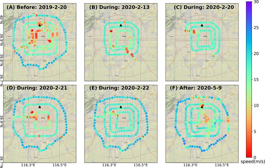
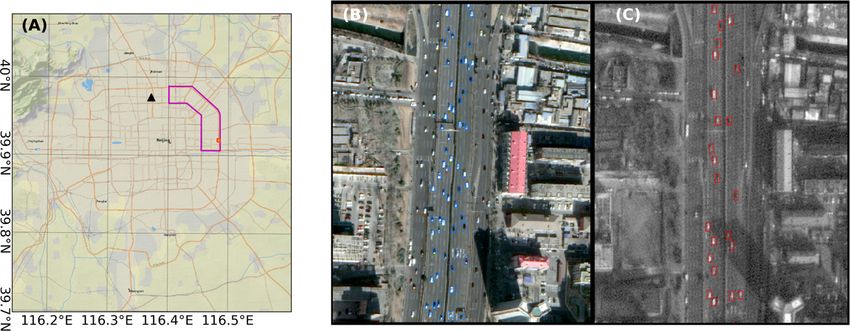
4602                                                            D. Liu et al.: Observed decreases in on-road CO2 concentrations

Figure 1. A: the locations of the second, third, fourth and fifth ring roads, the IAP tower (black triangle) and Olympic Sports Center station
(purple square); B1–B6: CO2 concentration at the IAP tower and PM2.5 concentration data from the Olympic Sports Center station during
six trips.

Figure 2. Photographs of the instrument installation for the on-road observations. (a–b) Picarro system installed in the vehicle; (c) low-cost
non-dispersive infrared (NDIR) sensors installed on the front windshield of the vehicle.

speed and altitude at 1 s resolution. These geographic in-               (also 21 % of the whole road). We used a visual interpreta-
formation data were averaged into 1 min intervals and then               tion method to obtain the numbers of vehicles on the third
matched with the CO2 concentration data according to time.               and fourth ring roads for BC and DC, respectively.
   Two remote sensing images were adopted (captured on                      To understand the traffic situation, we also collected the
21 February 2019 at 11:40:00 LST from a Google Earth                     real-time traffic congestion conditions (for each road), road
image, with 0.37 m spatial resolution; 19 February 2020                  name, geographic information, road type and average speed
at 10:20:08 LST from a Beijing-2 remote sensing satellite                as 1 h data from the AutoNavi open platform (https://lbs.
panchromatic image, with 0.8 m spatial resolution). Consid-              amap.com/, last access: May 2020).
ering the availability of data, we used the images from the
closest date and only part of the urban area. The comparison
region covered 10 km of the third ring road (accounting for
21 % of the whole road) and 13.4 km of the fourth ring road

Atmos. Chem. Phys., 21, 4599–4614, 2021                                                     https://doi.org/10.5194/acp-21-4599-2021
D. Liu et al.: Observed decreases in on-road CO2 concentrations                                                         4603

Table 1. Weather conditions during six trips.

       Label/date           Weather                  Air condition    Wind speed   PBLH    Real-time
       yyyy-mm-dd           condition              (PM2.5 : µg m3 )    (m s−1 )      (m)   panoramic photographs
       BC                   Clear day                           38       2.5       897.7
       2019-2-20 (Wed)

       DC                   Heavily polluted day               169       2.5         589
       2020-2-13 (Fri)

       DC                   Lightly polluted day               110       1.3         691
       2020-2-20 (Fri)

       DC                   Clear day                           12       2.5        1587
       2020-2-21 (Fri)

       DC                   Clear day                            6       3.6        1113
       2020-2-22 (Fri)

https://doi.org/10.5194/acp-21-4599-2021                                              Atmos. Chem. Phys., 21, 4599–4614, 2021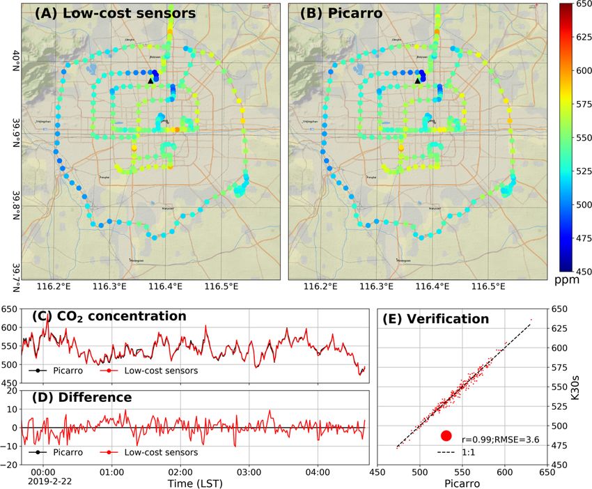
4604 D. Liu et al.: Observed decreases in on-road CO2 concentrations
Table 1. Continued.
Label/date Weather Air condition Wind speed PBLH Real-time
yyyy-mm-dd condition (PM2.5 : µg/m3 ) (m s−1 ) (m) panoramic photographs
AC Clear day 37 1.6 608
2020-5-9 (Sat)
Table 2. Instrument parameters for six on-road observations.
Label Date Instrument Accuracy Temporal resolution
(original → processed)
BC 2019-2-20 Picarro G2401 ±0.1 ppm 2 s → 1 min
DC
2020-2-13 LI-COR LI-7810 ±3.5 ppm (for 1 s);
2020-2-20 LI-COR LI-7810 improved into ±1 ppm 1 s → 1 min
2020-2-21 LI-COR LI-7810 (for 1 min)
2020-2-22 LI-COR LI-7810
AC 2020-5-9 Low-cost Sensor ±5 ppm 2 s → 1 min
(K30)
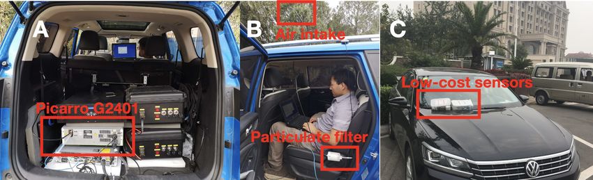
6 Results why the CO2 concentration was high on the innermost road
(second ring road) in Fig. 4a and d and on the outermost road
6.1 On-road CO2 concentration (fifth ring road) in Fig. 4f. The comparison of the three trips
indicated that the CO2 concentration in Fig. 4d was lower
than those in Fig. 4a and f, and the statistics show that the
The CO2 concentration maps of six on-road trips are shown
mean CO2 of the DC trips was approximately 58 (±1.1) and
in Fig. 4. According to Table 1, we selected four trips as the
46 (±6) ppm lower than those of the BC and AC trips, respec-
trips with the most similar weather conditions: one BC trip
tively. In addition, the average CO2 concentration observed at
(20 February 2019; Fig. 4a), two DC trips (21 and 22 Febru-
the IAP tower during the same periods was much lower than
ary 2020; Fig. 4d and e) and one AC trip (9 May 2020;
the on-road observations (Fig. 1B). These concentration dif-
Fig. 4f). Statistically, the average of the two DC trips was
ferences (gradients) also implied that ground transportation
444 (±1) ppm, which was 69 (±1.1) and 57 (±6) ppm lower
emissions were a major CO2 source on these urban roads.
than that of the BC and AC trips, respectively. The other
However, it was difficult to completely eliminate the im-
two DC trips (13 and 20 February) were conducted on
pact of background CO2 fluctuations only though selecting
(lightly/heavily) polluted days, and the CO2 concentrations
trips with the most similar weather conditions. For exam-
on these two days were as high as those during the BC and
ple, the PBLHs during two DC trips with the most similar
AC trips.
weather were 1587 and 1113 m, which were almost twice of
We chose one DC trip (21 February 2020) for further anal-
those during the BC and AC trips (Table 1). The CO2 concen-
ysis and compared it to the BC and AC trips. All three trips
trations at the IAP tower also indicated that during these two
were conducted on clear days, and their trajectories were
DC trips, the CO2 concentrations were 427 (±0.1) and 428
similar, from the outermost circle to the innermost circle, and
(±0.1) ppm, which were approximately 20 ppm lower than
covered one (morning or evening) rush hour. The difference
those for the BC and AC trips (in Fig. 1).
was that the BC and DC trips hit the evening rush hour on the
innermost ring road, whereas the AC trip hit the morning rush
hour on the outermost ring road. This difference explained
Atmos. Chem. Phys., 21, 4599–4614, 2021 https://doi.org/10.5194/acp-21-4599-2021
D. Liu et al.: Observed decreases in on-road CO2 concentrations                                                                      4605

Figure 3. Verification of low-cost sensors for on-road observations. (a) Map of CO2 concentrations measured by the low-cost sensor; (b)
map of the CO2 concentration measured by the Picarro system on the same vehicle; (c) time series of the CO2 concentrations measured by
the low-cost sensor and Picarro system; (d) difference (low-cost sensor concentration minus Picarro concentration); (e) scatter plot of the
low-cost sensor and Picarro data, with an RMSE of 3.6 ppm.

6.2   On-road CO2 enhancement                                           6.3   Diurnal variation analysis

To further reduce the influence of background CO2 varia-                Figure 6 shows the diurnal variation in the CO2 concentra-
tions, we calculated the CO2 enhancement for six trips by               tions from IAP tower observations, on-road CO2 concen-
subtracting the CO2 concentration at IAP tower from the on-             trations, enhancements and trajectories. In Fig. 6a, the CO2
road CO2 concentration (shown in Fig. 5). The spatial distri-           concentrations measured at the IAP tower were stable and
bution patterns of the enhancement were similar to the dis-             showed an approximate 50 ppm difference between trips.
tribution of the CO2 concentration maps, in which the en-               The CO2 concentrations at the IAP tower during the first
hancements during rush hours were much higher for all trips.            two DC trips (13 and 20 February 2020) were ∼ 30 ppm
Furthermore, the refined spatial distribution of the CO2 gra-           higher than those during the BC and AC trips. However,
dient implied emissions from ground transportation.                     the CO2 concentrations during the other two DC trips (21
   It is worth noting that the enhancements for the four DC             and 22 February 2020) were ∼ 20 ppm lower than those
trips were almost the same, although the weather conditions             during the BC and AC trips. These “baseline” CO2 con-
(based on the PBLH, PM2.5 and wind speed data) during                   centration fluctuations make the on-road observations not
these trips were quite different. However, the DC enhance-              directly comparable. In Fig. 7b, the CO2 concentrations
ments were obviously different from the BC and AC en-                   show a “double-peak” pattern, with peaks during the morn-
hancements. During the two DC trips on polluted days (13                ing (07:00–09:00 LST) and evening (17:00–20:00 LST) rush
and 20 February 2020), the mean CO2 concentrations were                 hours. During the rush hours, the CO2 concentrations ranged
similar to those during the BC and AC trips (Fig. 4b and c);            from 500 to 600 ppm, which were approximately 100 ppm
however, the enhancements extracted the traffic emission sig-           higher than the concentrations during working hours (09:00–
nals from the background, with averages of 33 (±1.1) and 16             17:00 LST). The comparison of BC and AC indicates that the
(±1.1) ppm (Fig. 5b and c). Statistically, the average of the           CO2 concentrations measured on 13 and 20 February 2020
four DC enhancements was 24 (±1.1) ppm, which was 41                    did not significantly decrease during 12:00–17:00 LST. How-
(±0.2) and 26 (±6.2) ppm lower than those of the BC and                 ever, the CO2 concentrations measured on 21 and 22 Febru-
AC enhancements.                                                        ary 2020 were much lower (∼ 50 ppm) than those measured

https://doi.org/10.5194/acp-21-4599-2021                                                  Atmos. Chem. Phys., 21, 4599–4614, 2021
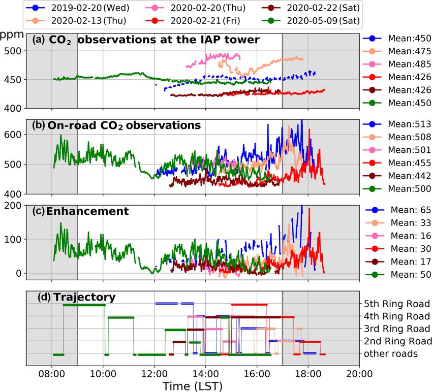
4606                                                          D. Liu et al.: Observed decreases in on-road CO2 concentrations

Figure 4. CO2 concentration maps for six on-road trips. Circles mark the locations of CO2 concentration records taken at a 1 min interval
(see methods). All subplots have the same color scale, ranging from 400 to 600 ppm. The black triangle is the location of the IAP tower.
One trip (a: 20 February 2019) was conducted before the COVID-19 restrictions, with an average of 513 (with an instrument uncertainty of
±0.1) ppm. Four trips (b–e: 13, 20, 21 and 22 February 2020) were conducted during COVID-19 restrictions, with averages of 508 (±1), 501
(±1), 455 (±1) and 442 (±1) ppm, respectively. One trip (f: 9 May 2020) was conducted after the COVID-19 restrictions, with an average
of 501 (±5) ppm.

Figure 5. Maps of the CO2 enhancement for all six trips calculated by subtracting the IAP tower measurements from the on-road CO2
measurements matched temporally. All subplots have the same color scale, ranging from −50 to 200 ppm. One trip (a: 20 February 2019)
was conducted before the COVID-19 restrictions, with an average of 65 (±0.2) ppm. Four trips (b–e: 13, 20, 21 and 22 February 2020) were
conducted during the COVID-19 restrictions, with averages of 33 (±1.1), 16 (±1.1), 30 (±1.1) and 17 (±1.1) ppm, respectively. One trip (f:
9 May 2020) was conducted after the COVID-19 restrictions, with an average of 50 (±5.1) ppm.

Atmos. Chem. Phys., 21, 4599–4614, 2021                                                   https://doi.org/10.5194/acp-21-4599-2021
D. Liu et al.: Observed decreases in on-road CO2 concentrations                                                               4607

during the BC and AC trips. This difference is consistent with    6.4    Analysis of CO2 enhancement for independent time
the spatial distribution mentioned before and is most likely             periods and roads
due to background CO2 fluctuations.
   In Fig. 6c, all DC enhancements were generally lower than      According to the previous analysis, we found that enhance-
the BC and AC enhancements, and the statistics for different      ment exhibited a strong correlation with time (rush or work-
time periods are listed in Table 3. However, we also found        ing hours) and road type. Therefore, we statistically analyzed
small enhancements for BC and AC, similar to those for DC.        the CO2 enhancement according to the road type and time
For example, the AC enhancement at 12:00–16:00 LST was            period, as shown in Fig. 7. In Fig. 7a, on 13 and 20 Febru-
almost the same as the DC enhancement at that time. By ex-        ary 2020, the CO2 concentrations on the other, second and
amining the trip routes (Fig. 6d), we found that during that      fourth, ring roads and all roads were at the same levels as
period, the on-road observation vehicle was not driving on        those during the BC and AC trips. However, in Fig. 7b, the
the main ring roads. As another example, the BC enhance-          four DC enhancements were generally lower than those dur-
ment at 18:00 LST indicates that the enhancement decreased        ing AC and BC for all road types. Although on the sec-
in a stepwise manner, also because the vehicle drove on other     ond ring road, the DC enhancements on 13 and 21 Febru-
roads (Fig. 6d).                                                  ary 2020 were almost the same as the BC and AC enhance-
   The mean enhancement for the whole BC trip was 65              ments, the DC trips were during rush hours, whereas the AC
(±0.2) ppm, and the average for the evening rush hours            and BC trips were during working hours. Some very high de-
(100 ± 0.2 ppm) was 2 times that for the working hours            viations also occurred (rush hours on the other roads: second
(54 ± 0.2 ppm). This result implies that the increase in vehi-    and fifth ring roads), which indicates the dispersion of the
cle volume during the evening rush hours leads to large traffic   CO2 enhancement. The reason for this difference is that we
emissions and an increase in the on-road CO2 concentration.       classified all roads excluding the ring roads as other roads,
For DC, all trips covered the working hours, with a low en-       which may have included arterial and residential roads, so
hancement of approximately 20 ppm. There was no obvious           the different road types may have increased the deviation.
difference between weekdays and weekends during working           For the second and fifth ring roads, high deviation occurred
hours. The reason may be that the government encouraged           because during rush hour, traffic flow and transportation var-
people to work remotely at home. Therefore, even on week-         ied greatly and resulted in drastic changes in the CO2 en-
days, according to traffic conditions, the commute volume         hancement, which also caused much higher deviations. After
was low (Fig. S2). Among these four trips, two (on 13 and         a statistical significance test, we found that the CO2 enhance-
20 February 2020) covered the evening rush hours with high        ment difference between working times and rush hours for
averaged enhancements of 55 (±1.1) and 50 (±1.1) ppm.             all trips was significant (p
4608                                                                       D. Liu et al.: Observed decreases in on-road CO2 concentrations

Table 3. CO2 enhancement (mean and instrumental uncertainties) for six trips over different periods (ppm). Times are indicated in LST.

         Label                  Observation          Weather                   Total               Morning             Working               Evening
                                date                 condition                average            rush hours             hours              rush hours
                                                                           (07:00–20:00)      (07:00-09:00)         (09:00–17:00)      (17:00–20:00)
         BC                     2019-2-20 (Wed)      Clear                  65 (±0.2)                         –       54 (±0.2)           100 (±0.2)
         DC
                                2020-2-13 (Thu)      Stable/heavy           33 (±1.1)                         –       26 (±1.1)               55 (±1.1)
                                                     pollution
                                2020-2-20 (Thu)      Stable/light           16 (±1.1)                         –       16 (±1.1)                       –
                                                     pollution
                                2020-2-21 (Fri)      Windy day              30 (±1.1)                         –       16 (±1.1)               50 (±1.1)
                                2020-2-22 (Sat)      Windy day              17 (±1.1)                         –       17 (±1.1)                       –
         AC                     2020-5-9 (Sat)       Windy day              50 (±5.1)              80 (±5.1)          46 (±5.1)                       –
         Total BC–DC                                                        41 (±1.3)                         –       35 (±1.3)               48 (±1.3)
         Total AC–DC                                                        26 (±6.2)                         –       27 (±6.2)                       –

Table 4. Statistical analysis (mean value and 1 standard deviation) of the CO2 enhancement for six trips according to the time and road type.

       Label   Date                 Time            Other    Second ring    Third ring   Fourth ring   Fifth ring       All          Significance
                                                    roads          road          road          road         road      roads            test (p)
                                                                                                                              Working hours       DC/AC
                                                                                                                               compared to     compared to
                                                                                                                                 rush hours           BC
       BC
               2019-2-20 (Wed)      Working hours   31/24         81/26        77/11         56/18         37/8      54/26                                –
                                                                                                                                      0.015
                                    Rush hours      58/37        125/34             –             –            –    100/48                                –
                                    Both            42/33        109/38        77/11         56/18         37/8      65/38               –                –
       DC
               2020-2-13 (Thu)      Working hours    8/16         29/15        38/13         29/11             –     26/18                                –
                                                                                                                                      0.018
                                    Rush hours      10/14         74/20        37/14              –            –     55/31                                –
                                    Both             9/16         63/28        38/13         29/11             –     33/26               –           0.041
               2020-2-20 (Thu)      Working hours    9/13           15/8       14/10           24/8            –     16/11               –                –
                                    Rush hours         –              –             –             –            –         –                                –
                                    Both             9/13           15/8       14/10           24/8            –     16/11               –           0.001
               2020-2-21 (Fri)      Working hours   12/13             –             –        25 ± 7       13 ± 7    16 ± 10                               –
                                                                                                                                      0.002
                                    Rush hours      32/17         67/29             –        35/15             –     50/28                                –
                                    Both            20/18         67/29             –        30/13         13/7      30/26               –           0.026
               2020-2-22 (Sat)      Working hours   16/11           22/7         21/8        15/13             –     17/12               –                –
                                    Rush hours         –              –             –             –            –         –                                –
                                    Both            16/11           22/7         21/8        15/13             –    17 ± 12              –           0.001
       AC
               2020-5-9 (Sat)       Working hours   30/22         65/18        60/14         57/17        73/18      46/26                                –
                                                                                                                                      0.008
                                    Rush hours      89/28             –             –             –       75/24      81/26                                –
                                    Both            36/29         65/18        60/14         57/17        73/20      50/28               –            0.41

Atmos. Chem. Phys., 21, 4599–4614, 2021                                                                    https://doi.org/10.5194/acp-21-4599-2021
D. Liu et al.: Observed decreases in on-road CO2 concentrations 4609 Figure 6. The six trips were plotted on a single day. The two gray regions refer to the morning and evening rush hours. The six colorful lines represent the six trips on different days. Four of the six trips covered at least one (morning and/or evening) rush hour. Panel (a) shows the CO2 concentration at the IAP tower during the trips. Panel (b) shows the on-road CO2 concentration. Panel (c) shows the CO2 enhancements. Panel (d) shows the six trip trajectories. Figure 7. Statistical analysis (mean and 1 standard deviation) of all on-road trips according to the road types and times. Panel (a) shows the on-road CO2 concentration. Panel (b) shows the CO2 enhancement. https://doi.org/10.5194/acp-21-4599-2021 Atmos. Chem. Phys., 21, 4599–4614, 2021
4610                                                       D. Liu et al.: Observed decreases in on-road CO2 concentrations

ysis of road traffic operation in Beijing during COVID-19 in           dard deviations shown in Table 4 mainly presented CO2
2020” published by the Beijing Transport Institute, during             concentration fluctuations within specific periods and
the first 8 weeks (from 1 February to 31 March, the DC pe-             on certain roads and uncertainty from instruments (rel-
riod in this study), the Beijing ground transportation index           atively small).
(calculated based on the ratio of congested road length to the
whole road length) decreased by 53 % compared to that on            2. The IAP tower CO2 concentration was used as the
normal days, whereas, from 1 April to 31 May, the index re-            background from Beijing. In this study, the IAP tower
covered to 92 % (Zhang, 2020). The index implied that traf-            data were adopted as the urban background CO2 con-
fic flow for DC was dramatically decreased compared to that            centration in Beijing. Its measurement footprint was
for BC, and the index for AC almost recovered but not com-             influenced by two factors: wind speed/direction and
pletely. This index variation is consistent with our observa-          air intake height. For wind speed/direction, in Beijing,
tions. Second, two remote sensing images from similar dates            the main wind directions were northwest (winter) and
were adopted (Fig. 8). According to statistics and estimations         southeast (summer) (Cheng et al., 2018). Generally,
based on coverage area, we found that the BC traffic flows on          high-level data have a large footprint and good repre-
the main roads of the fourth and third ring roads were 227 and         sentativeness. For example, Cheng et al. (2018) showed
226 veh km−1 (vehicles per kilometer), respectively. How-              that CO2 data recorded at 280 m height have an average
ever, the DC traffic flow decreased to 35 and 34 veh km−1 , re-        fetch of ∼ 17 km, which covers a major part of the city;
flecting a reduction of approximately 85 %. With the assum-            data collected at 80 m height have an average fetch of
ing that emission factors were the same, the CO2 emissions             ∼ 8 km; data collected at 8 m height may have an aver-
on roads for DC may have sharply decreased by approxi-                 age fetch of only ∼ 230 m; and the fetch at the surface
mately 85 % compared to those for BC. This difference is               (2 m) may be smaller. Therefore, there are two uncer-
higher than the passenger transportation decrease estimated            tainties. The first is the height variation during the ob-
by Han et al. (2020) (56 % in the first quarter of 2020) be-           servation trips. Due to the data availability and for com-
cause remote sensing images are snapshots and cover only               parison consistency, we chose the lower- and surface-
part of the urban area. Moreover, Hans’ results are the aver-          level data. According to Cheng et al. (2018), the CO2
age of the first 3 months and the entire Beijing administrative        concentration at the 80 m height is ∼ 15 ppm higher
region. Third, we also used traffic congestion condition data,         than that at the 8 m height. Therefore, if this difference
although with low temporal and spatial resolution, to indi-            between the lower level and surface level was added,
cate the on-road traffic flow and emissions (Fig. 9). Fourth,          the BC enhancement would increase (∼ 15 ppm), which
the vehicle speed maps of the six trips were plotted (Fig. 10).        means that the DC enhancement would be even lower
Overall, these maps reflect the spatial patterns of road traf-         (∼ 56 ppm) than the BC enhancement. The other is the
fic conditions during the surveys and could also reflect the           difference between the surface-level data and 280 m
specifics on a single road. However, these maps are sensi-             height data in different seasons. According to Cheng
tive to subjective speed variations caused by drivers, such as         et al. (2018), the monthly averaged CO2 showed a rel-
when facing traffic lights.                                            atively stable difference among the different heights:
                                                                       the CO2 at the lower level was approximately 40 ppm
7.2    Uncertainty analysis                                            higher than that at 280 m in February and approximately
                                                                       30 ppm higher in May. The AC enhancement should in-
In this research, uncertainty mainly existed in the following          crease 10 ppm additionally, which means that the DC
terms:                                                                 enhancement would be even lower (∼ 36 ppm) than the
 1. Uncertainty existed from the observation instruments.              AC enhancement. Considering these uncertainties, the
    In this study, four instruments were adopted for measur-           results support our hypothesis.
    ing CO2 concentrations: three for on-road observations
    (a Picarro G2401, with an accuracy of approximately             3. Influences of vegetation sinks and natural changes were
    0.1 ppm; a LI-COR LI-7810, ∼ 1 ppm; and a low-cost                 also prevalent. To understand the CO2 variability im-
    sensor, no more than 5 ppm) and one for the IAP                    pacted by natural sinks (especially for vegetation), we
    tower observation (Picarro G2301, ∼ 0.1 ppm). Dur-                 used the dynamic vegetation and terrestrial carbon cycle
    ing analysis, both the proposed enhancement method                 model VEGAS (Zeng et al., 2014) to simulate the terres-
    and the CO2 concentration or enhancements of differ-               trial biosphere–atmosphere flux (Fta) in Beijing during
    ent trips were compared using linear analysis (addition            2000–2020 (Fig. S3). The model was run at a 2.5 × 2.5◦
    or subtraction). Therefore, the enhancement uncertain-             resolution from 1901 to June 2020, forced by observed
    ties from the observation instruments were ∼ 0.2 ppm               climate variables, including monthly precipitation and
    for BC, ∼ 1.1 ppm for DC, less than 5.1 ppm for AC,                hourly temperature. Although precipitation and temper-
    ∼ 1.3 ppm for comparing BC and DC, and less than                   ature in 2020 were higher than the climatology (aver-
    6.2 ppm for comparing DC and AC. Note that the stan-               age of the last 20 years), the difference between the Fta

Atmos. Chem. Phys., 21, 4599–4614, 2021                                            https://doi.org/10.5194/acp-21-4599-2021
D. Liu et al.: Observed decreases in on-road CO2 concentrations 4611
Figure 8. Traffic volume comparison with using remote sensing images. (a) Coverage region of remote sensing images (purple polygon)
and example region shown on the right (red square); (b) remote sensing images from Google Earth on 21 February 2019 at 11:42:00 LST,
with a spatial resolution of 0.37 m for multispectral band images; 61 vehicles on the main road were interpreted (labeled by blue polygons);
(c) remote sensing image from the Beijing-2 satellite on 19 February 2020 at 10:20:08 LST, with a spatial resolution of 0.8 m for the
panchromatic band images and 24 vehicles labeled with red polygons.
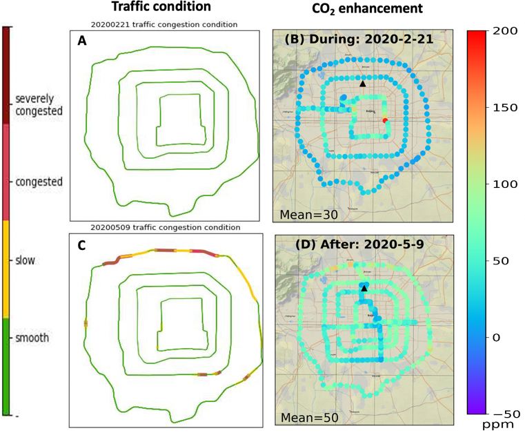
Figure 9. Comparison of traffic conditions with the CO2 enhancement. (a) Traffic conditions on 21 February 2020; (b) CO2 enhancement
on 21 February 2020; (c) traffic conditions on 9 May 2020; (d) CO2 enhancement on 9 May 2020.
in 2020 and the average was within 1 standard devia- 2016). The results (Fig. S4) showed that the background
tion. This suggests that the Fta in 2020 was not obvi- CO2 concentration variation mainly induced by natural
ously unusual compared to that over the last 20 years. factors from February to May was only approximately
We also analyzed the CO2 concentration at the Shang- 5 ppm. However, these two factors (vegetation flux and
dianzi station in the Beijing rural region, which is one natural changes) both indicate areas far larger than Bei-
of the three WMO/GAW regional stations in China, to jing urban areas. Because the location of the IAP tower
determine the CO2 background variation (Fang et al., and the tracks of the on-road observations are both in
https://doi.org/10.5194/acp-21-4599-2021 Atmos. Chem. Phys., 21, 4599–4614, 20214612 D. Liu et al.: Observed decreases in on-road CO2 concentrations
Figure 10. Speed maps of six trips, ranging from 0 to 30 m s−1 . One trip (a: 20 February 2019) was conducted before the COVID-19
restrictions. Four trips (b–e: 13, 20, 21 and 22 February 2020) were conducted during the COVID-19 restrictions; one trip (f: 9 May 2020)
was conducted after the COVID-19 restrictions.
urban Beijing and we used the enhancement method, and weather. However, the enhancement metric, which was
these factors were reduced. the difference in the on-road CO2 concentration and the city
“background”, reduced the impact of background CO2 fluc-
4. When data were collected, especially when switching tuations. The results showed that for DC, the total average
between lower and upper levels, a large amount of data CO2 enhancements of the four trips were 41 (±1.3) ppm and
was lost. However, because the data gaps were evenly 26 (±6.2) ppm lower than those for BC and AC, respectively.
distributed and the IAP tower CO2 concentrations were Detailed analysis showed that this reduction commonly ex-
relatively stable, we assumed that it would not affect the isted on all road types during the same time period (rush
final statistical results. hours/working hours). For the DC trips, there was no sig-
nificant difference during work hours between weekdays and
5. In this study, our on-road observations did not have a weekends. The enhancements during rush hours were much
fixed route or beginning/ending time, which means that higher than those during working hours, and compared with
the observations on different dates represented different the enhancement reduction during rush hours for BC, that for
roads. Therefore, we analyzed a wide time range of ob- DC was more obvious. Our findings, which show a clear de-
servations (rush hours, working hours or whole days), crease for DC compared with BC and AC, are consistent with
which may have also caused uncertainty. the COVID-19 restrictions, which may be direct evidence of
reductions in CO2 concentrations and carbon emissions. On-
road CO2 observations are an effective way to understand
8 Conclusion and analyze the urban carbon CO2 concentration distribution
and variation and should be regularly and more frequently
The CO2 emission reduction caused by COVID-19 restric-
conducted in future work. The development and successful
tions is an opportunity to test our ability to collect CO2 obser-
application of the miniaturized and low-cost CO2 monitoring
vations in urban areas. In this study, we chose on-road CO2
instruments used in this study (Khan et al., 2012; Shusterman
concentrations as the target, because ground transportation is
et al., 2016; Martin et al., 2017; Müller et al., 2020; Bao et
the main source of CO2 in urban areas and was remarkably
al., 2020) will greatly aid in the collection of on-road obser-
influenced by policy restrictions due to the COVID-19 pan-
vations and even high-density network observations and play
demic. We conducted six on-road observations in Beijing,
a key role in future urban carbon observations.
including one trip before COVID-19 restrictions, in Febru-
ary 2019; four trips during COVID-19 restrictions, in Febru-
ary 2020; and one trip in May 2020, after COVID-19 restric-
tions had been eased. The results showed that on-road CO2
concentrations were strongly affected by traffic emissions
Atmos. Chem. Phys., 21, 4599–4614, 2021 https://doi.org/10.5194/acp-21-4599-2021D. Liu et al.: Observed decreases in on-road CO2 concentrations 4613
Code availability. The scripts used in this study are open and can Friedlingstein, P., Jones, M. W., O’Sullivan, M., Andrew, R. M.,
be made available to interested users upon contacting the corre- Hauck, J., Peters, G. P., Peters, W., Pongratz, J., Sitch, S., Le
sponding author. Quéré, C., Bakker, D. C. E., Canadell, J. G., Ciais, P., Jack-
son, R. B., Anthoni, P., Barbero, L., Bastos, A., Bastrikov, V.,
Becker, M., Bopp, L., Buitenhuis, E., Chandra, N., Chevallier,
Data availability. The data in this study are open and can be made F., Chini, L. P., Currie, K. I., Feely, R. A., Gehlen, M., Gilfillan,
available to interested users upon contacting the corresponding au- D., Gkritzalis, T., Goll, D. S., Gruber, N., Gutekunst, S., Har-
thor. ris, I., Haverd, V., Houghton, R. A., Hurtt, G., Ilyina, T., Jain,
A. K., Joetzjer, E., Kaplan, J. O., Kato, E., Klein Goldewijk, K.,
Korsbakken, J. I., Landschützer, P., Lauvset, S. K., Lefèvre, N.,
Supplement. The supplement related to this article is available on- Lenton, A., Lienert, S., Lombardozzi, D., Marland, G., McGuire,
line at: https://doi.org/10.5194/acp-21-4599-2021-supplement. P. C., Melton, J. R., Metzl, N., Munro, D. R., Nabel, J. E. M. S.,
Nakaoka, S.-I., Neill, C., Omar, A. M., Ono, T., Peregon, A.,
Pierrot, D., Poulter, B., Rehder, G., Resplandy, L., Robertson, E.,
Rödenbeck, C., Séférian, R., Schwinger, J., Smith, N., Tans, P. P.,
Author contributions. PH, BY and NZ conceived and designed the
Tian, H., Tilbrook, B., Tubiello, F. N., van der Werf, G. R., Wilt-
study. DL summarized the results and wrote the draft of the pa-
shire, A. J., and Zaehle, S.: Global Carbon Budget 2019, Earth
per. WS and PH designed and conducted the on-road observations.
Syst. Sci. Data, 11, 1783–1838, https://doi.org/10.5194/essd-11-
PW provided the IAP tower observation data. KZ, ZL, HM and QC
1783-2019, 2019.
helped to collect, process and analyze data.
George, K., Ziska, L. H., Bunce, J. A., and Quebedeaux, B.: El-
evated atmospheric CO2 concentration and temperature across
an urban-rural transect, Atmos. Environ., 41, 7654–7665,
Competing interests. The authors declare that they have no conflict https://doi.org/10.1016/j.atmosenv.2007.08.018, 2007.
of interest. Grimmond, C. S. B., King, T. S., Cropley, F. D., Nowak, D. J., and
Souch, C.: Local-scale fluxes of carbon dioxide in urban environ-
ments: methodological challenges and results from Chicago, En-
Acknowledgements. Special thanks are given to Zhe Hu, Zhimin viron. Pollut., 116, S243–S254, https://doi.org/10.1016/s0269-
Zhang and Xiaoli Zhou for collecting the data and conducting the 7491(01)00256-1, 2002.
observations. Gross, B., Zheng, Z., Liu, S., Chen, X., Sela, A., Li, J., Li, D.,
and Havlin, S.: Spatio-temporal propagation of COVID-19 pan-
demics, arXiv [preprint], https://arxiv.org/abs/2003.08382 (last
Financial support. This research has been supported by the Min- access: May 2020), arXiv:2003.08382, 2020.
istry of Science and Technology of the People’s Republic of China Han, P., Cai, Q., Oda, T., Zeng, N., Shan, Y., Lin, X., and Liu, D.:
(grant no. 2017YFB0504000). Assessing the recent impact of COVID-19 on carbon emissions
from China using domestic economic data, Sci. Total Environ.,
750, 141688, https://doi.org/10.1016/j.scitotenv.2020.141688,
Review statement. This paper was edited by Ralf Sussmann and re- 2020.
viewed by two anonymous referees. Idso, C. D., Idso, S. B., and Balling, R. C.: The urban
CO2 dome of Phoenix, Arizona, Phys. Geogr., 19, 95–108,
https://doi.org/10.1080/02723646.1998.10642642, 1998.
Idso, C. D., Idso, S. B., and Balling, R. C.: An intensive two-
References week study of an urban CO2 dome in Phoenix, Arizona, USA,
Atmos. Environ., 35, 995–1000, https://doi.org/10.1016/s1352-
Bao, Z., Han, P., Zeng, N., Liu, D., Cai, Q., Wang, Y., Tang, 2310(00)00412-x, 2001.
G., Zheng, K., and Yao, B.: Observation and modeling of Idso, S. B., Idso, C. D., and Balling, R. C.: Seasonal and diurnal
vertical carbon dioxide distribution in a heavily polluted sub- variations of near-surface atmospheric CO2 concentration within
urban environment, Atmos. Ocean. Sci. Lett., 13, 371–379, a residential sector of the urban CO2 dome of Phoenix, AZ, USA,
https://doi.org/10.1080/16742834.2020.1746627, 2020. Atmos. Environ., 36, 1655–1660, https://doi.org/10.1016/s1352-
Bush, S. E., Hopkins, F. M., Randerson, J. T., Lai, C.-T., and 2310(02)00159-0, 2002.
Ehleringer, J. R.: Design and application of a mobile ground- Khan, A., Schaefer, D., Tao, L., Miller, D. J., Sun, K., Zondlo, M.
based observatory for continuous measurements of atmospheric A., Harrison, W. A., Roscoe, B., and Lary, D. J.: Low Power
trace gas and criteria pollutant species, Atmos. Meas. Tech., 8, Greenhouse Gas Sensors for Unmanned Aerial Vehicles, Remote
3481–3492, https://doi.org/10.5194/amt-8-3481-2015, 2015. Sens., 4, 1355–1368, https://doi.org/10.3390/rs4051355, 2012.
Cheng, X. L., Liu, X. M., Liu, Y. J., and Hu, F.: Char- Kutsch, W., Vermeulen, A., Karstens, U.: Finding a hair in the
acteristics of CO2 Concentration and Flux in the Bei- swimming pool: the signal of changed fossil emissions in the
jing Urban Area, J. Geophys. Res.-Atmos., 123, 1785–1801, atmosphere, available at: https://www.icos-cp.eu/event/917, last
https://doi.org/10.1002/2017jd027409, 2018. access: December 2020.
Fang, S. X., Tans, P. P., Dong, F., Zhou, H., and Luan, T.: Character- Le Quere, C., Jackson, R. B., Jones, M. W., Smith, A. J. P., Aber-
istics of atmospheric CO2 and CH4 at the Shangdianzi regional nethy, S., Andrew, R. M., De-Gol, A. J., Willis, D. R., Shan, Y.,
background station in China, Atmos. Environ., 131, 1–8, 2016.
https://doi.org/10.5194/acp-21-4599-2021 Atmos. Chem. Phys., 21, 4599–4614, 20214614 D. Liu et al.: Observed decreases in on-road CO2 concentrations Canadell, J. G., Friedlingstein, P., Creutzig, F., and Peters, G. Picarro G2301 Analyzer Datasheet: https://www.picarro. P.: Temporary reduction in daily global CO2 emissions during com/support/library/documents/g2301_analyzer_datasheet? the COVID-19 forced confinement, Nat. Clim. Change, 10, 647– language=en# (last access: 20 June 2020), 2019. 653, https://doi.org/10.1038/s41558-020-0797-x, 2020. Rosenzweig, C., Solecki, W., Hammer, S. A., and Mehrotra, S.: LI-COR LI-7810 Brochure: https://www.licor.com/documents/ Cities lead the way in climate-change action, Nature, 467, 909– yldtj3q6jykx3xnc8680ytx6i0afc9uu (last access: 20 June 2020), 911, https://doi.org/10.1038/467909a, 2010. 2019. SenseAir: K30 products sheets: https://rmtplusstoragesenseair.blob. Liu, Z., Ciais, P., Deng, Z., Lei, R., Davis, S. J., Feng, S., Zheng, core.windows.net/docs/publicerat/PSP110.pdf (last access: 20 B., Cui, D., Dou, X., Zhu, B., Guo, R., Ke, P., Sun, T., Lu, C., July 2020), 2019. He, P., Wang, Y., Yue, X., Wang, Y., Lei, Y., Zhou, H., Cai, Z., Shusterman, A. A., Teige, V. E., Turner, A. J., Newman, C., Kim, J., Wu, Y., Guo, R., Han, T., Xue, J., Boucher, O., Boucher, E., and Cohen, R. C.: The BErkeley Atmospheric CO2 Observation Chevallier, F., Tanaka, K., Wei, Y., Zhong, H., Kang, C., Zhang, Network: initial evaluation, Atmos. Chem. Phys., 16, 13449– N., Chen, B., Xi, F., Liu, M., Bréon, Lu, Y., Zhang, Q., Guan, 13463, https://doi.org/10.5194/acp-16-13449-2016, 2016. D., Gong, P., Kammen, D. M., He, K., and Schellnhuber, H. J.: Su, T., Li, Z., and Kahn, R.: Relationships between the plan- Near-real-time monitoring of global CO2 emissions reveals the etary boundary layer height and surface pollutants derived effects of the COVID-19 pandemic, Nat Commun, 14, 11, 5172, from lidar observations over China: regional pattern and in- https://doi.org/10.1038/s41467-020-18922-7, 2020. fluencing factors, Atmos. Chem. Phys., 18, 15921–15935, Martin, C. R., Zeng, N., Karion, A., Dickerson, R. R., Ren, https://doi.org/10.5194/acp-18-15921-2018, 2018. X., Turpie, B. N., and Weber, K. J.: Evaluation and envi- Sun, W., Deng, L., Wu, G., Wu, L., Han, P., Miao, Y., ronmental correction of ambient CO2 measurements from a and Yao, B.: Atmospheric Monitoring of Methane in Bei- low-cost NDIR sensor, Atmos. Meas. Tech., 10, 2383–2395, jing Using a Mobile Observatory, Atmosphere-Basel, 10, https://doi.org/10.5194/amt-10-2383-2017, 2017. https://doi.org/10.3390/atmos10090554, 2019. Mitchell, L. E., Lin, J. C., Bowling, D. R., Pataki, D. E., Strong, Sussmann, R. and Rettinger, M.: Can We Measure a COVID-19- C., Schauer, A. J., Bares, R., Bush, S. E., Stephens, B. B., Related Slowdown in Atmospheric CO2 Growth? Sensitivity of Mendoza, D., Mallia, D., Holland, L., Gurney, K. R., and Total Carbon Column Observations, Remote Sens., 12, 2387, Ehleringer, J. R.: Long-term urban carbon dioxide observations https://doi.org/10.3390/rs12152387, 2020. reveal spatial and temporal dynamics related to urban charac- Woodwell, G. M., Houghton, R. A., and Tempel, N. R.: Atmo- teristics and growth, P. Natl. Acad. Sci. USA, 115, 2912–2917, spheric CO2 at Brookhaven, Long-Island, New-York – Patterns https://doi.org/10.1073/pnas.1702393115, 2018. of Variation up to 125 Meters, J. Geophys. Res., 78, 932–940, Müller, M., Graf, P., Meyer, J., Pentina, A., Brunner, D., Perez- https://doi.org/10.1029/JC078i006p00932, 1973. Cruz, F., Hüglin, C., and Emmenegger, L.: Integration and cali- Zeng, N., Zhao, F., Collatz, G. J., Kalnay, E., Salawitch, R. J., West, bration of non-dispersive infrared (NDIR) CO2 low-cost sensors T. O., and Guanter, L.: Agricultural Green Revolution as a driver and their operation in a sensor network covering Switzerland, At- of increasing atmospheric CO2 seasonal amplitude, Nature, 515, mos. Meas. Tech., 13, 3815–3834, https://doi.org/10.5194/amt- 394–397, https://doi.org/10.1038/nature13893, 2014. 13-3815-2020, 2020. Zhang, Y.: Analysis of road traffic operation in Beijing during Ott, L., Peters, G., and Meyer, A.,: Special virtual panel: Covid- COVID-19 in 2020, available at: https://mp.weixin.qq.com/s/ 19 and its impact on global carbon emissions, https://carbon. AtSXWtK4LvzI7UPuJTHvIQ, last access: August 2020 (in Chi- nasa.gov/policy_speaker_28052020.html (last access: Decem- nese). ber 2020. Zhang, Z., Wong, M., and Lee, K.: Estimation of potential source Perez, I. A., Luisa Sanchez, M., Angeles Garcia, M., and regions of PM2.5 in Beijing using backward trajectories, Atmos. de Torre, B.: CO2 transport by urban plumes in the up- Pollut. Res., 6, 173–177, https://doi.org/10.5094/apr.2015.020, per Spanish plateau, Sci. Total Environ., 407, 4934–4938, 2015. 10.1016/j.scitotenv.2009.05.037, 2009. Zheng, J., Dong, S., Hu, Y., and Li, Y.: Comparative anal- Picarro G2401 Analyzer Datasheet: https://www.picarro. ysis of the CO2 emissions of expressway and arterial com/support/library/documents/g2401_analyzer_datasheet? road traffic: A case in Beijing, Plos One, 15, e0231536, language=en# (last access: 20 July 2020), 2017. https://doi.org/10.1371/journal.pone.0231536, 2020. Atmos. Chem. Phys., 21, 4599–4614, 2021 https://doi.org/10.5194/acp-21-4599-2021
You can also read