Critical Transitions in Public Opinion: A Case Study of American Presidential Election - arXiv

Critical Transitions in Public Opinion: A Case Study of American Presidential
 Election

 Ning Ning Chung1,2, Lock Yue Chew1,2* and Choy Heng Lai3,‡

Affiliations: 1Complexity Institute, Nanyang Technological University Singapore 637973
2
 School of Physical & Mathematical Sciences, Nanyang Technological University Singapore
637377
3
 Department of Physics, National University of Singapore, Singapore 117551
Correspondence to: *lockyue@ntu.edu.sg and ‡phylaich@nus.edu.sg

Abstract:
At the tipping point, it is known that small incident can trigger dramatic societal shift. Getting
early-warning signals for such changes are valuable to avoid detrimental outcomes such as riots
or collapses of nations. However, it is notoriously hard to capture the processes of such
transitions in the real-world. Here, we demonstrate the occurrence of a major shift in public
opinion in the form of political support. Instead of simple swapping of ruling parties, we study
the regime shift of a party’s popularity based on its attractiveness by examining the American
presidential elections during 1980-2012. A single irreversible transition is detected in 1991. Once
a transition happens, recovery to the original level of attractiveness does not bring popularity of
the political party back. Remarkably, this transition is corroborated by tell-tale early-warning
signature of critical slowing down. Our approach is applicable to shifts in public attitude within
any social system.

Main Text:
Complex systems are known to undergo critical changes (1-8). Classic examples in this respect
are natural ecosystems, where collapse has been observed in the fisheries stocks, in global
climate change, and the bleaching of the coral reefs. It is usual for such critical transition to be
triggered by a gradual perturbation or a seemingly minor happenstance. Once the transition
begins, it can become drastic with an impact that is abrupt and irreversible. Interestingly, theory
which governs ecosystem regime shifts has wide applicability. It has recently been applied even
to the banking system (9-11). Shifts between alternate stable states have also been shown
theoretically in social (12) and coupled socio-ecological systems (13). More empirical evidences
are however needed to validate their existence in these systems. It is in these contexts that critical
transition is demonstrated in this report in social systems of general interest. Here, we show how
a model of opinion dynamics is directly applicable to recent American presidential elections with
critical transitions predicted theoretically and duly verified empirically.
Opinions are dynamic and are heavily influenced by the underlying social interaction
mechanisms. A notable mechanism is peers' influence, where individuals tend to follow the

social opinion of their peers (14, 15). In consequence, they are more likely to adopt the opinion
of the majority (16). There is also the situation where an individual persists on its opinion
regardless of the views of its social environment. Such individuals are known as zealots (17, 18).
However, few studies have been conducted on the intrinsic capacity of an opinion in affecting
the choice of an individual. In this case, the opinion is deemed to bear a set of basic attributes
which characterizes its quality and renders it appealing for adoption. We term this the
attractiveness of the opinion.
Here, we introduce a theoretical model on two competing opinions R and D. The model
incorporates all the three mechanisms discussed above: majority rule; inertial to make social
change; and implicit attractiveness of the opinion. Let us represent the agents of our social
system by a network of size N with average degree k. A fraction fR (fD) of the N agents are
selected randomly to stick firmly to opinion R (D) with fR + fD ≤ 1, and these agents are zealots.
The rest of the agents are flexible and they select their opinions by making their choice either
through the majority-rule or the attractiveness of the opinion. At each time step, a flexible agent
is randomly chosen to update its opinion. There is a probability pm for the selected agent to
decide based on the majority-rule. In this case, the agent adopts the opinion followed by the
majority of its peers. Conversely, the agent has a probability of 1 - pm to decide with respect to
the opinion’s attractiveness. When this happens, it adopts opinion R with probability AR and
opinion D with probability AD such that AR + AD = 1. We start our investigation on the system
dynamics with a large AR. The system is allowed to evolve for a sufficiently long time until it
reaches steady state. After which, the steady-state value for the fraction of agents that adopt
opinion R, i.e. PR, is recorded. The value of AR is then gradually decreased. For each decrement
of AR, we record PR. The process is then reversed by gradually increasing AR to its original value.
This would give us the dynamical changes of opinion R as its attractiveness varies from large to
small and then back to its original value.
Depending on the value of pm, AR, fR and fD, different opinion dynamics as exhibited by the PR -
AR plot is observed (see Fig. 2). When pm = 0, PR and AR follows a monotically increasing one-to-
one linear relationship. However, this functional behavior becomes nonlinear as pm is increased,
where we observe the occurrence of a sharp transition between opinions. Beyond a critical pm,
the transition transforms further. We observe the interesting phenomenon of hysteresis and
irreversible behaviour. The horizontal width of the hystereis loop that emerges is found to
increase as we continue to increase pm. We expect PR = fR when AR = 0, and PR = 1 - fD when AR
= 1.
Thus, a fundamental and unexpected outcome of the model is critical and irreversible transition
of the dominance of the opinion from one to the other. It arises from the interplay between the
mechanisms of majority rule and opinion's attractiveness. As the attractiveness of opinion R (AR)
increases from the state where opinion D is dominant (in the direction of single arrow in Fig 2e),
the adoption of opinion R increases. But this increase is restrained below the level possible from
a monotonic linear increase in lieu that opinion D is the majority. By symmetry, the same
argument applies when we reduce AR (which is equivalent to an increase in opinion D's
attractiveness, AD, and in the direction of the double arrow in Fig. 2e) from the state when R is
dominant. This explains why there is a sharp nonlinear change in between that accounts for the
sudden switch of opinions. More significantly, this switch in opinion can occur at different AR in
the forward and backward direction, leading to irreversible behavior and hysteresis loop.

 2

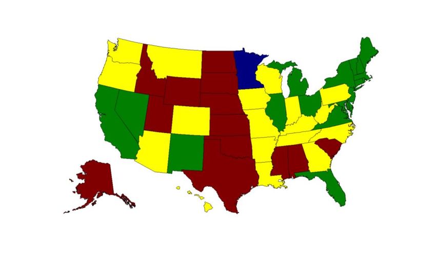
While scientific investigation of presidential election has already been performed in various
contexts (15, 19, 20), we hypothesize that our simple model possesses the main social
mechanisms that drive the American presidential election. The American presidential election is
held every four years via state elections. Each of the fifty states, plus Washington DC, is
allocated with a certain number of electoral votes. In most states (except Maine and Nebraska),
all allocated electoral votes are to be won through the majority votes. There are a total of 538
electoral votes and accomplishing a sum of 270 electoral votes (or more) in states' victory is all a
president need to win an election. Interestingly, as we examine the American election results
from 1980 to 2008 (21), we observe a ubiquitous and yet distinct voting pattern from states with
different historical and social background. 13 of the states are found to be unfailingly
Republican, while Minnesota and the districts of Columbia always vote for the Democrat during
the period under study. The rest are swing states which sometimes vote for the Republican but
other times for the Democrat.
We first examine the behavior of voters from the 13 Republican-committed states, which are
shown in red in Fig. 1. A proxy for AR is defined based on the average vote for the Republican
candidate for these 13 states (see Methods). Notably, we observe that the votes obtained by the
Republican candidates in each of these states possess a simple increasing monotonic relationship
with our surrogate AR, for example, in Texas, Idaho and Wyoming (see Fig 2(a) – (c)). These
results correspond to our model when pm is small and indicates that the average vote is a good
measure of the attractiveness of a Republican candidate. Incidentally, this average vote reflects
not only the attractiveness of R in the Republican-committed states, it also implies the
attractiveness of the Republican candidate in the Democrat-committed states, which is consistent
with the outcome of our model. Votes obtained by the Republican in Minnesota, a Democratic
state (shown in blue in Fig. 1), is found to increase linearly with the increase of AR as shown in
Fig. 2(d).
In contrast, votes for swing states are found to depend nonlinearly on AR. Let us take California
as an example. While the Republican votes there may look random and unpredictable for a given
attractiveness as shown in Fig. 2(e), the results become meaningful by following the history of
the state election carefully. It reveals the interesting phenomenon of hysteresis as in the model.
California was initially (1980-1988) a Republican-dominated state. The Republican votes in
California were higher in 1984 as R is more attractive in that year than 1980 and 1988. The
Republican lost a large number of its followers as its attractiveness decreases over the four-year
period when George Bush was the president of America. By the 1992 election, the Republican
had become very unattractive and had a very low following in California. The critical transition
from being popular to unpopular is observed to be hysteretic and irreversible. Eight years later in
the 2000 election, the Republican had managed to regain its popularity in Texas and a few
others, but not in California. Note that such an irreversible transition is also observed in 17 other
swing states shown in green in Fig. 1. It is however not observed in the states which are colored
yellow in Fig. 1.
It is significant that the above empirical observations correspond to the PR - AR relationship for
each state obtained from our model. This implies that we can match theory to data through
calibrating the parameters pm, fR and fD. The results are illustrated in Fig. 2. Good correspondence
is found for all the states (see Supplementary Material for the rest of the states).
Critical slowing down precedes critical transition. It gives the most important clue (22-26) and
early warning that the system is getting close to the transition point. During the period of our

 3

study from 1980 to 2008, we detect its symptom (see Fig. 3) in 1991, which is one year before
the 1992 election, through the presidential approval rating (PAR). Note that political analysts
(27) have identified PAR as a good global indicator on election outcome. The result here is
consistent with our observation above, as critical slowing down is found to occur just prior to the
period of critical irreversible transition in the support of the Republican during the tenure of
George Bush. When a system is close to the transition point, the rate of recovering from small
perturbation is lower, and its dynamics is characterized by high correlation and large standard
deviation as shown in Fig. 3(b).
Let us next test our model by using it to predict the 2012 election. In order to make prediction,
our model requires a measure on the perception of the candidate at the population level. For this,
we shall use PAR in conjunction with a new quantity ⟨ ⟩ for our prediction. ⟨ ⟩ (⟨ ⟩) is the
average fraction of votes for the 51 electoral colleges cast in favor of the Republican
(Democratic) candidate for each election year. The appropriateness of ⟨ ⟩ is discerned from its
close correspondence to the PAR (except when there was a change in the incumbent political
party in the year 2000 and 2008 elections, see Fig. 3). Specifically, we observe that ⟨ ⟩ ≈ PAR
when the president is a Republican, and ⟨ ⟩ ≈ 1 - PAR when the president is a Democrat since
⟨ ⟩ = 1 - ⟨ ⟩. We can easily compute the relationship between ⟨ ⟩ and AR by making use of
the 51 PR - AR relations that was determined earlier. The ⟨ ⟩ - AR relation is necessary to predict
the outcome of future presidential election.
For the 2012 election, we use 1 - PAR = 49.9 (with 50.1 being the PAR on October 2012 of
President Obama) to make prediction. Among the 51 electoral colleges, election results for three
of the states, namely Florida, Virginia and Colorado are found to be the least predictable (see
Fig. S7) because the statistical error of their PR is larger than their winning margin. Notably,
these three states are among the seven super-swingy states identified by Sabato et. al. in their
2016 electoral map (28). Our predictions for the Republican votes from our model are shown in
Table 1. On average, we observe a discrepancy of 2.7% between the predicted and the actual
votes. This has led to a difference of 13 electoral votes between the results of our prediction (219
EV) and those based on the actual election (206 EV).
The popularity level between the Democratic candidate Hillary Clinton and the Republican
candidate Donald Trump has been tracked by RealClearPolitics (29) since May 2015. While the
favorability rating of Clinton is way ahead of Trump initially, their gap has finally closed
recently after much fluctuations, with Clinton slightly ahead with a spread of 4. Interestingly,
president Obama’s approval rating has remain at around 52 according to opinion polls performed
by Gallup in Sep 2016 (30). If this rating persists till November 2016, the Republican could end
up losing the election with an electoral vote that ranges between 175 and 228 (see Table S1). On
the other hand, competition between the two parties can become far more intense if the
Republican candidate is able to acquire a ⟨ ⟩ of 51.7 which would enable them to win the
election. In this case, the votes for the two parties would be extremely close in the 11 states
marked red in Table S1.

 4

Methods

Proxy for Attractiveness
The proxy for attractiveness ARj is obtained based on the average vote for the Republican
candidate for the 13 Republican-committed states ̅ of the j-th election as follows:
 = ̅ − 0.5 ⟨| ̅ − ̅ |⟩ .
In order for this proxy not to be too far off from the average vote over the 51 electoral states ̅ ,
we have subtracted a constant term 0.5 ⟨| ̅ − ̅ |⟩ which represents the mean discrepancy
between the two average votes over the eight election years.

L2 Error
The L2 error is defined as follows:

 2 = √∑ ( − )2 .

Note that vjM is the vote determined from our model, while vjD is the actual vote obtained
empirically. Both are for the j-th election.

 5

Figure 1: Classification of US states based on voting patterns at state election level held between
1980 and 2008. States are categorized into Republican-committed states (red), Democratic-
committed states (blue), swing states in which hysteresis are observed (green) and swing states in
which hysteresis are not observed (yellow).

 6

Figure 2: Dependence of the fraction of vote for the Republican candidate PR on its attractiveness
AR for 8 American states. Empirical election results are shown as filled circles with the size of
the circle increases with the year of the election. Results from our model are shown as solid line.
Here, critical points for figures (e) to (h) are estimated from 40 simulations with standard
deviations ranging from 0.02 to 0.04.

 7

Figure 3: (a) The presidential approval rating (PAR) for American presidents from 1980 to 2016.
Note that PAR are shown as it is for the Republican presidents (red curve), but for Democratic
presidents, 1-PAR are shown instead (blue curve). The Republican votes (averaged over 51
electoral colleges), i.e. ⟨ ⟩, are shown as circles for comparison. Autocorrelation lagged by
seven days are shown for presidential approval rating between (b) Mar 1991 and Oct 1991, (c)
Jan 1999 and Aug 1999, (d) Feb 2007 and Oct 2008, (e) Sep 2015 and Apr 2016. Critical
slowing down is observed as an indicator that the system is near to the ‘tipping point’ in 1991.

(a)

(b) (c)

 8

(d) (e)

Table 1. Prediction of the election results based on the Oct 2012 Presidential Approval Rating of
1-PAR = 49.9. Note that the average vote for the Republican candidate in the 2012 election is
49.0.

 2012 Election Model Discrepancy
Electoral College
 Vote EV Vote EV Vote EV
1. Alabama 60.5 9 57.6 9 -2.9 0
2. Alaska 54.8 3 60.0 3 +5.2 0
3. Arizona 53.7 11 56.4 11 +2.7 0
4. Arkansas 60.6 6 54.9 6 -5.7 0
5. California 37.1 - 40.6 - +3.5 0
6. Colorado 46.1 - 48.9 - +2.8 0
7. Connecticut 40.7 - 43.1 - +2.4 0
8. Delaware 40.0 - 42.4 - +2.4 0
9. Dist. Of Col. 7.3 - 10.7 - +3.4 0
10. Florida 49.1 - 48.5 - -0.6 0
11. Georgia 53.3 16 55.1 16 +1.8 0
12. Hawaii 27.8 - 37.3 - +9.5 0
13. Idaho 64.5 4 65.6 4 +1.1 0
14. Illinois 40.7 - 40.5 - -0.2 0
15. Indiana 54.1 11 56.9 11 +2.7 0
16. Iowa 46.2 - 48.4 - +2.2 0
17. Kansas 59.7 6 59.4 6 -0.3 0
18. Kentucky 60.5 8 58.0 8 -2.5 0
19. Louisiana 57.8 8 55.2 8 -2.6 0
20. Maine 41.0 - 42.4 - +1.4 0
21. Maryland 35.9 - 40.0 - +4.1 0
22. Massachusetts 37.5 - 33.7 - -3.8 0
23. Michigan 44.7 - 47.5 - +2.8 0

 9

24. Minnesota 45.0 - 45.6 - +0.6 0
25. Mississippi 55.3 6 57.0 6 +1.7 0
26. Missouri 53.8 10 52.4 10 -1.4 0
27. Montana 55.4 3 55.8 3 +0.4 0
28. Nebraska 59.8 5 63.9 5 +4.1 0
29. Nevada 45.7 - 44.6 - -1.1 0
30. New Hampshire 46.5 - 46.8 - +0.3 0
31. New Jersey 40.6 - 40.6 - 0.0 0
32. New Mexico 42.8 - 44.9 - +2.1 0
33. New York 35.2 - 38.1 - +2.9 0
34. North Carolina 50.4 15 53.7 15 +3.3 0
35. North Dakota 58.3 3 60.7 3 +2.4 0
36. Ohio 47.7 - 46.8 - -0.9 0
37. Oklahoma 66.8 7 62.5 7 -4.3 0
38. Oregon 42.1 - 45.6 - +3.5 0
39. Pennsylvania 46.7 - 47.9 - +1.2 0
40. Rhode Island 35.2 - 33.7 - -1.5 0
41. South Carolina 54.6 9 57.3 9 +2.7 0
42. South Dakota 57.9 3 58.1 3 +0.2 0
43. Tennessee 59.5 11 55.6 11 -3.9 0
44. Texas 57.2 38 58.6 38 +1.4 0
45. Utah 72.8 6 68.3 6 -4.5 0
46. Vermont 31.0 - 35.6 - +4.6 0
47. Virginia 47.3 - 51.7 13 +4.4 +13
48. Washington 41.3 - 46.7 - +5.4 0
49. West Virginia 62.3 5 55.6 5 -6.7 0
50. Wisconsin 46.0 - 48.4 - +2.4 0
51. Wyoming 68.6 3 65.4 3 -3.2 0
 Total 206 219 13

 10

References:
1. Scheffer M, Carpenter S, Foley JA, Folke C, Walker B (2001) Catastrophic Shifts in
Ecosystems. Nature 413: 591.
2. Scheffer M, Carpenter S, Lenton T, Bascompte J, Brock W, Dakos V, van de Koppel J,
Leemput I, Levin S, van Nes E, Pascual M, Vandermeer J (2012) Anticipating Critical
Transitions. Science 338(6105): 344-348.
3. Tripati A, Backman J, Elderfield H, Ferretti P (2005) Eocene bipolar glaciation associated
with global carbon cycle changes. Nature 436: 341-346.
4. Liu Z, et al. (2009) Global cooling during the Eocene-Oligocene climate transition. Science
323: 1187-1190.
5. Barnosky AD, et al. (2012) Approaching a State Shift in Earth’s Biosphere. Nature 486: 52.
6. Kefi S, Rietkerk M, Alados CL, Pueyo Y, Papanastasis, VP, Elaich A, Ruiter PC (2007)
Spatial Vegetation Patterns and Imminent Desertification in Mediterranean Arid Ecosystems.
Nature 449: 213.
7. Rietkerk M, Dekker SC, de Ruiter PC, van de Koppel J (2004) Self-organized patchiness and
catastrophic shift in ecosystems. Science 305: 1926-1929.
8. Christianen MJA, et al. (2014) Habitat collapse due to overgrazing threatens turtle
conservation in marine protected areas. Proc R Soc B 281: 2890.
9. May RM, Levin S, Sugihara G (2008) Ecology for Bankers. Nature 451: 893.
10. Haldane AG, May RM (2011) Systemic Risk in Banking Ecosystems. Nature 469: 351.
11. Kambhu J, Weidman S, Krishnan N (2007) New Directions for Understanding Systemic Risk
(National Academies Press, Washington DC). Also published as Econ Policy Rev 13: 2.
12. Ohta M, Iida T, Kawaoka T (1995) Opinion Transition Model under Dynamic Environment:
Experiment in Introducing Personality to Knowledge-based Systems. Industrial and Engineering
Applications of Artificial Intelligence and Expert Systems: p. 569-574.
13. Lade SJ, Tavoni A, Levin S, Schlüter M (2013) Regime Shift in a Social-ecological System.
Theoretical Ecology 6: 359-372.
14. Liggett TM (1985) Interacting Particle System (Springer, New York).
15. Fernández-Gracia J, Suchecki K, Ramasco JJ, Miguel MS, Eguíluz VM (2014) Is the Voter
Model a Model for Voters? Physical Review Letters 112: 158701.
16. Galam S (2002) Minority Opinion Spreading in Random Geometry. European physics
Journal B 25: 403-406.
17. Crokidakis N, Oliveira PMC (2015) Inflexibility and Independence: Phase transitions in the
Majority-rule Model. Physical Review E 92: 062122.
18. Waagen A, Verma G, Chan K, Swami A, D'Souza RM (2015) Effect of Zealotry in High-
dimensional Opinion Dynamics Models. Physical Review E 91: 022811.
19. Fortunato S, Castellano C (2007) Scaling and Universality in Proportional Elections.
Physical Review Letters 99: 138701.

 11

20. Klimek P, Yegorov Y, Hanel R, Thurner S (2012) Statistical Detection of Systematic
Election Irregularities. Proc Natl Acad Sci USA 109: 16469-16473.
21. Source: The American Presidency Project.
22. van Nes EH, Scheffer M (2007) Slow recovery from perturbations as generic indicator of a
nearby catastrophic shift. Am Nat 169(6): 738-747.
23. Scheffer M, et al. (2009) Early-warning signals for Critical Transitions. Nature 461(7260):
53-59.
24. Drake JM, Griffen BD (2010) Early Warning Signal of Extinction in Deteriorating
Environments. Nature 467(7314): 456-459.
25. Dai L, Korolev KS, Gore J (2013) Slower Recovery in Space Before Collapse of Connected
Populations. Nature 496: 355.
26. Leemput IA, et al. (2014) Critical Slowing Down as Early Warning for the Onset and
Termination of Depression. Proc Natl Acad Sci USA 111: 87-92.
27. Kyle K, Geoffrey S, Sabato LJ (2015) Clinton’s Real Opponent: Barack Obama. Politico
April 17.
28. Kyle K, Geoffrey S, Sabato LJ (2015) The 2016 Results We Can Already Predict. Politico
May 3.
29. Source: http://www.realclearpolitics.com
30. Source: http://www.gallup.com

Author contributions: All authors contributed equally.

 12

Supplementary Materials:

Figure S1: Dependence of the fraction of vote for the Republican candidate PR on its
attractiveness AR. The relations are shown here for 8 states with hysteresis.

 13

Figure S2: Dependence of the fraction of vote for the Republican candidate PR on its
attractiveness AR. The relations are shown here for 6 states with hysteresis.

 14

Figure S3: Dependence of the fraction of vote for the Republican candidate PR on its
attractiveness AR. The relations are shown here for 8 states without hysteresis.

 15

Figure S4: Dependence of the fraction of vote for the Republican candidate PR on its
attractiveness AR. The relations are shown here for 7 states without hysteresis.

 16

Figure S5: Dependence of the fraction of vote for the Republican candidate PR on its
attractiveness AR. The relations are shown here for 8 states without hysteresis.

 17

Figure S6: Dependence of the fraction of vote for the Republican candidate PR on its
attractiveness AR. The relations are shown here for 6 states without hysteresis.

 18

Figure S7: Statistical analysis performed on our model to determine its predictability on winning
of the state election based on 1 - PAR = 49.9. In order to predict a win at the state level, the L2
error of the estimate of the vote should be less than four times the winning margin M, where M =
|PR – PD|. We have taken a stricter criterion of L2 error = 2M as the boundary for predictability.

 19

Figure S8: Further check on the validity of our model by examining the relationship between the
number of acquired electoral votes and ⟨ ⟩. Good correspondence is observed between model
and data not only on the direct relationship between these variables, but also on the occurrence of
historical precedence in their relationships, except for the election years: 1980, 1992, 1996 and
2000, where the presence of an independent candidate is not negligible. Note that the dashed line
(solid line) represents votes obtained before (after) transition of opinions from our model. The
circle marker denotes election results derived empirically. The electoral votes are allocated based
on the 2010 Census which is effective for the 2012, 2016 and 2020 American presidential
elections.

 20

Table S1. Prediction of the 2016 election results based on an average vote for the Republican
candidate ⟨ ⟩ of 51.7 and 48.

 With average vote of 51.7 With average vote of 48
Electoral College
 Vote EV Vote EV
1. Alabama 58.7 9 56.2 9
2. Alaska 61.7 3 58.0 3
3. Arizona 58.0 11 53.9 11
4. Arkansas 56.8 6 52.6 6
5. California 43.6 - 39.8 -
6. Colorado 50.4 9 47.1 -
7. Connecticut 44.1 - 41.1 -
8. Delaware 46.8 - 40.1 -
9. Dist. Of Col. 10.8 - 10.4 -
10. Florida 51.9 29 44.2 -
11. Georgia 56.1 16 53.5 16
12. Hawaii 38.9 - 35.2 -
13. Idaho 67.5 4 63.8 4
14. Illinois 41.6 - 39.9 -
15. Indiana 58.1 11 55.0 11
16. Iowa 49.8 - 46.4 -
17. Kansas 61.0 6 57.3 6
18. Kentucky 58.8 8 56.1 8
19. Louisiana 56.8 8 53.0 8
20. Maine 46.6 - 40.1 -
21. Maryland 40.8 - 39.0 -
22. Massachusetts 34.4 - 32.9 -
23. Michigan 50.2 16 44.3 -
24. Minnesota 46.8 - 43.7 -
25. Mississippi 57.8 6 55.9 6
26. Missouri 54.3 10 49.9 -
27. Montana 57.7 3 53.4 3
28. Nebraska 65.4 5 62.1 5
29. Nevada 47.9 - 41.6 -
30. New Hampshire 51.5 4 42.3 -
31. New Jersey 43.6 - 39.8 -
32. New Mexico 49.0 - 42.4 -
33. New York 39.0 - 37.4 -
34. North Carolina 55.1 15 52.0 15
35. North Dakota 62.2 3 58.7 3
36. Ohio 49.9 - 45.3 -
37. Oklahoma 64.1 7 60.6 7

 21

38. Oregon 47.4 - 43.4 -
39. Pennsylvania 49.0 - 46.4 -
40. Rhode Island 34.4 - 32.9 -
41. South Carolina 58.2 9 56.1 9
42. South Dakota 59.5 3 55.8 3
43. Tennessee 56.7 11 54.8 11
44. Texas 60.1 38 56.6 38
45. Utah 69.9 6 66.5 6
46. Vermont 36.4 - 34.8 -
47. Virginia 55.0 13 47.8 -
48. Washington 48.4 - 44.2 -
49. West Virginia 57.2 5 53.8 5
50. Wisconsin 49.8 - 46.4 -
51. Wyoming 67.0 3 63.6 3
 Total 277 196

 22