Cryogenic Trapped-Ion System for Large Scale Quantum Simulation
←
→
Page content transcription
If your browser does not render page correctly, please read the page content below
Cryogenic Trapped-Ion System for Large Scale
                                           Quantum Simulation
                                                  G. Pagano1 , P.W. Hess2 , H. B. Kaplan1 , W. L. Tan1 , P.
arXiv:1802.03118v1 [quant-ph] 9 Feb 2018

                                                  Richerme3 , P. Becker1 , A. Kyprianidis1 , J. Zhang1 , E.
                                                  Birckelbaw1 , M. R. Hernandez1 , Y. Wu4 and C. Monroe1,5
                                                  1
                                                    Joint Quantum Institute, Department of Physics and Joint Center for Quantum
                                                  Information and Computer Science, University of Maryland, College Park, MD 20742
                                                  2
                                                     Middlebury College Department of Physics, Middlebury, VT 05753
                                                  3
                                                     Department of Physics, Indiana University, Bloomington, IN 47405
                                                  4
                                                     Department of Physics, University of Michigan, Ann Arbor, MI 48109
                                                  5
                                                     IonQ Inc., College Park, MD 20740

                                                  Abstract. We present a cryogenic ion trapping system designed for large scale
                                                  quantum simulation of spin models. Our apparatus is based on a segmented-blade ion
                                                  trap enclosed in a 4 K cryostat, which enables us to routinely trap over 100 171 Yb+
                                                  ions in a linear configuration for hours due to a low background gas pressure from
                                                  differential cryo-pumping. We characterize the cryogenic vacuum by using trapped
                                                  ion crystals as a pressure gauge, measuring both inelastic and elastic collision rates
                                                  with the molecular background gas. We demonstrate nearly equidistant ion spacing
                                                  for chains of up to 44 ions using anharmonic axial potentials. This reliable production
                                                  and lifetime enhancement of large linear ion chains will enable quantum simulation of
                                                  spin models that are intractable with classical computer modelling.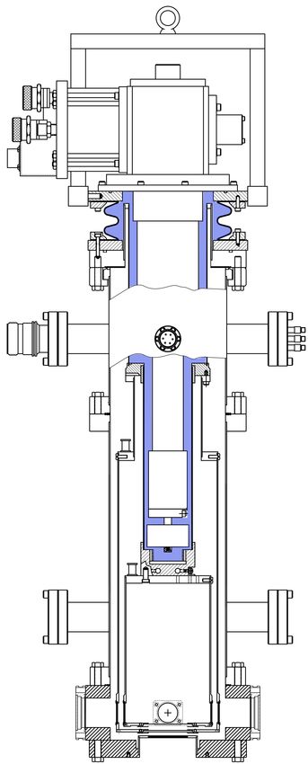
Cryogenic Trapped-Ion System for Large Scale Quantum Simulation                         2

1. Introduction

Atomic ions confined in radio-frequency (rf) Paul traps are the leading platform for
quantum simulation of long-range interacting spin models [1, 2, 3, 4, 5]. As these
systems become larger, classical simulation methods become incapable of modelling
the exponentially growing Hilbert space, necessitating quantum simulation for precise
predictions. Currently room temperature experiments at typical ultra-high-vacuum
(UHV) pressures (10−11 Torr) are limited to about 50 ions due to collisions with
background gas that regularly destroy the ion crystal [6]. The background pressure
achievable in UHV vacuum chambers is ultimately limited by degassing of inner surfaces
of the apparatus. However, cooling down the system to cryogenic temperatures turns
the inner surfaces into getters that trap most of the residual background gases. This
technique, called cryo-pumping, has led to the lowest level of vacuum ever observed
(< 5 · 10−17 Torr) [7].
     Here we report an experimental setup consisting of a macroscopic segmented blade
trap into a cryogenic vacuum apparatus that allows for the trapping and storage of large
chains of ions. In section 2 we describe the system design, focusing on the cryostat, the
helical resonator supplying the radio-frequency (rf) drive to the ion trap, and the atomic
source. In section 3 we report on the performance of the vibration isolation system and
the improvements to the mechanical stability of the whole structure inside the 4 K
region. In section 4 we show pressure measurements using the ion crystals themselves
as a pressure gauge below 10−11 Torr. We characterize the dependence of the pressure
on the cryostat temperature by measuring the inelastic and elastic collision rates of
trapped ions with background H2 molecules. In section 5 we show the capability to
shape the axial potential in order to minimize the ion spacing inhomogeneity in large
ion chains, and in section 6 we summarize perspectives for future experiments.

2. The Apparatus

The challenge of merging atomic physics and ion trap technology with cryogenic
engineering has been successfully undertaken by many groups around the world
[8, 9, 10, 11, 12, 13, 14]. Cryogenic ion traps offer two remarkable advantages: Firstly,
heating rates [15, 16] due to surface patch potential and electric field noise can be
suppressed by orders of magnitude compared with room temperature traps, as it was
first demonstrated in [9]. Secondly, the low pressures achievable via cryo-pumping reduce
the collision rate with the residual background gas, thereby enhance the lifetime of the
ions in the trap. Indeed, in standard UHV systems, the storage time of a large number
of ions in a linear chain is typically limited by the probability that a “catastrophic”
collision event causes the ion crystal to melt and the ions to be ejected from the trap.
Assuming that the collisional loss probability scales linearly with the number of ions,
it is necessary to achieve a significant reduction in the background pressure in order
to increase the capabilities of the trapped-ion quantum simulator platform. Recent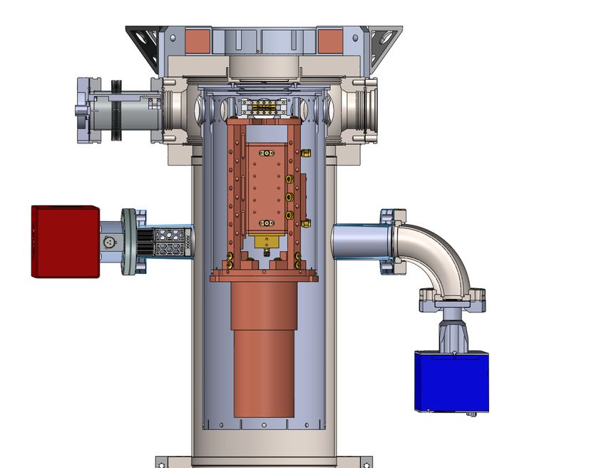
Cryogenic Trapped-Ion System for Large Scale Quantum Simulation                                                                               3
           High pressure                  Cold head
 a)         helium lines                                        b)
                                                                                                   Resonator
                                                                      SAES                          antenna
                                           Rubber
                                                                     NextTorr
                                           bellows                    D100

              Electrical                        rf electrical
            feedthrough                        feedthrough

                                                                                                                                 Pressure
                                                                            z        Helical                                       gauge
                                              Helium                                resonator                                   (not shown)
87.3 cm

                          Wire               exchange
                         anchor                 gas                                                                             Resonator
                                                                     x          y
                          posts             40 K stage                                                                           support
               Vacuum
                                                                                                                                structure
                jacket
                40 K                      Cold finger
               shield

                                             4 K stage
                 4K
                shield                                                    Oven
             Viewport                       1’’ Windows with
              flange                           teflon holder

          Spherical                               2.25’’
          octagon                            Reentrant window             Vertical magnetic coil          Heater   Blade trap

                                  Figure 1. Cryogenic vacuum apparatus. a) Side view section of the cryostat
                                  (courtesy of Janis Inc). b) Cross section view of the lower section, 90o rotated with
                                  respect to a). The vertical magnetic coil is mounted on the bottom of the reentrant
                                  window flange. An aluminium fixture with heaters held on it is designed to rest in the
                                  coil’s inner diameter in order to avoid water condensation on the outside face of the
                                  recessed window, when the apparatus is at 4 K.

pioneering techniques such as titanium coating and heat treatment [17] have been shown
to achieve extreme-high vacuum (XHV) in room temperature vacuum systems. However,
combining room temperature XHV with an ion trap apparatus remains a challenge
because many components in the vacuum system may not be XHV-compatible, such
as the common electrical insulators (Kapton or PEEK). On the other hand, with a
cryogenic setup, beside a lower residual gas density with respect to UHV systems, there
is the additional advantage of having a lower temperature residual background gas. For
this reason, the ion-molecule collisions, even when they occur, are not harmful for the
ion chain. Moreover, a cryogenic ion-trap apparatus can offer a significant background
pressure reduction at 4 K while maintaining high optical access for ion addressing
and detection. Therefore, careful design is required in order to: (a) minimize room
temperature blackbody radiation without limiting optical access and (b) mechanically
decouple the system from the cold head vibrations while maintaining significant cooling
power at 4 K. The design and the performance of the cryogenic apparatus will be
described in the next subsections.

2.1. The Cryostat
In order to minimize the vibrations induced by the cryocooler, one possible choice is a
flow cryostat [13] or a bath cryostat, which feature very low acoustic noise. However,
these types of cryostats require continuous replenishment of cold liquid coolant, which
is expensive and time-consuming. The alternative is to use a closed-cycle cryocooler
which does not require liquid coolant to be constantly refilled and it is more convenient
300
4K stage
Cryogenic Trapped-Ion System for Large Scale Quantum4K stage
Simulation 4
250
300
50Kstage
4K stage
Temperature [K]
200
50K
4K4K stage
stage stage
150 250 Resonator
50K
50K
40K stage stage
Resonator
50K stage
Temperature [K]
100 Resonator
200
50
Trap Mount
Resonator
Trap Mount 4K stage
150 Trap Mount
Resonator 50K stage
0
0 100
1 2 3 4 5 6 7 Trap Mount Resonator
50
time [hours]
Trap Mount Trap Mount
1 2 3 4 05 6 7
1 2 3 [hours]
time 4 05 1 62 3 74 5 6 7
1 2 3
time [hours] 4 5 6 7
time [hours]
1 2 3 [hours]
time 4 5 6 7
Figure 2. Typical cool-down cycle. The trap mount reaches a steady state
time [hours]temperature of 4.7 K while the equilibrium temperature of the helical resonator is
slightly higher (∼ 5.5 K) because of the reduced thermal contact with the 4 K stage.
The acceleration at the end of the cool-down is due to the steep decrease in copper
specific heat below 100 K [18].
as it only needs external electric supply. However, a closed cycle cryocooler suffers from
severe acoustic noise. To address this challenge, we decided to use a closed cycle Gifford-
McMahon cryostat, whose vibrating cold finger is mechanically decoupled from the main
vacuum apparatus through an exchange gas region (see Fig. 1a) filled with helium gas at
a pressure of 1 psi above atmosphere. The helium gas serves as a thermal link between
the cold finger and the sample mount to which the ion trap apparatus is attached.
A rubber bellows is the only direct mechanical coupling between the vibrating cold
head and the rest of the vacuum apparatus which is sitting on the optical breadboard.
This vibration isolation system allows us to keep the vibrations rms amplitude below
70 nm (see section 3 for more details). During normal operation, the vibrating cold
head is attached to the overhead equipment racks hanging from the ceiling and the
vacuum apparatus is resting on an optical breadboard. However, by connecting the cold
head and the cryostat mechanically, the entire system can be hoisted and moved from
the optical breadboard to a freestanding structure where upgrades and repairs can be
performed.
On top of the Cryostat (SHV-4XG-15-UHV), made by Janis Inc., sits a cold head
(SRDK-415D2) that is powered by a F-70L Sumitomo helium compressor. The cold
head features two stages with different cooling powers, 45 W for the 40 K stage and
1.5 W for the 4 K stage. In order to shield the ion trap apparatus from room temperature
blackbody radiation (BBR), two aluminium concentric cylindrical radiation shields are
in thermal contact with the two stages. Their BBR heat loads, estimated using the
Stephan-Boltzmann law ‡, are Q̇40K ∼ 5.5 W and Q̇4K ∼ 550 µW, well below the
‡ The radiation heat load Q̇ on a given surface S at temperature T0 from an environment at T1 isCryogenic Trapped-Ion System for Large Scale Quantum Simulation 5
cooling power of the two heat stages.
The thermal heat load on the trap due to the electrical wiring is estimated to
be negligible (∼ 100 µW) since the temperature probes (Lakeshore DT670A1-CO), the
static electrodes, and the ovens wires are all heat sunk to anchor posts (see Fig. 1a) in
good thermal contact with both stages. The four SMA cables connected to the radio-
frequency (rf) electrical feedthrough are not heat sunk and deliver an estimated heat
load of 500 mW and 220 mW on the 40 K and 4 K stages, respectively §. In designing
the apparatus, a good balance between room temperature BBR heat load and optical
access has been achieved, given the total cooling power. The spherical octagon (see
Fig. 1) features eight 1” diameter windows which provide optical access in the x-y
plane, held by soft teflon holders. On the bottom, the system features a 2.25” diameter
reentrant window which allows for a numerical aperture (NA) up to 0.5 to image the
ions along the vertical (z) direction. The whole cryostat rests on an elevated breadboard
to allow for ion imaging from underneath. The total heat load of the recessed window is
estimated to be 2.4 W on the 40 K shield and 1.7 mW on the 4 K shield. The total heat
load budget (see Appendix A) is well below the total cooling power, and therefore we
can cool the system down to 4.5 K in about 5 hours (see Fig. 2) with both the helical
resonator and the ion trap inside the 4 K shield.
Before the cool down, the apparatus is pre-evacuated using a turbo-molecular pump
until the pressure reading on the MKS-390511-0-YG-T gauge (not shown in Fig. 1b)
reaches the pressure of about ' 2 · 10−5 Torr. The gauge is attached through an elbow
in order to avoid direct “line of sight” exposure of its radiative heat load (1.5 W) to the
40 K shield. Since hydrogen is the least efficiently cryo-pumped gas, we added a SAES
NexTorr D-100 getter and ion pump (see Fig. 1b) which is attached to one of four CF40
flanges of the long bellow cross.
2.2. Blade trap
The blade-style ion trap was hand-assembled and aligned under a microscope with
' 5 µm resolution. The blades are made of alumina and have five segments. They were
cleaned with hydrofluoric acid and plasma ashed on both sides, then coated with a 100
nm titanium adhesion layer and a 1 µm gold layer at Sandia Laboratories. The coating
was applied by means of multi-directional evaporation to avoid alumina exposure in
the 50 µm wide gaps between the segments. The two static electrode blades are gold
coated with masks so that the five segments can be biased independently, whereas the
rf blades have an unsegmented coating. Gold ribbons (0.015” wide and 0.001” thick)
are wire-bonded on top of the blades for electrical connections. In order to shunt rf
given by the Stephan-Boltzmann law and it is proportional to Q̇ = σ(T14 − T04 )/V where σ = 5.67 · 10−8
W/(K4 ·m2 ) and V is the so called view, which is a function of the geometry, the surface S and their
emissivities.
RT
§ The heat conduction contribution of the wiring has been estimated as Q̇ = A/L T12 λ(T )dT , where A
is the wire cross-section, L is the wire length and λ(T ) is the temperature dependent heat conductivity
and T1 and T2 are the temperatures of the two ends of the wire [18]Cryogenic Trapped-Ion System for Large Scale Quantum Simulation 6
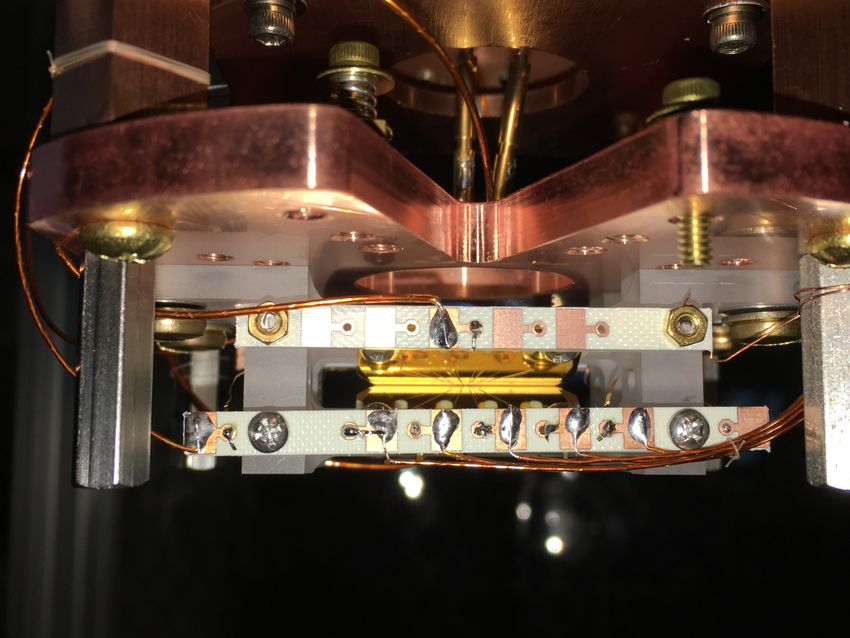
RF blade
Trap mount
Ground Sapphire holder Static blade Gold ribbon Copper pads
Figure 3. Blade ion trap. The blades are mounted on a sapphire holder and gold
ribbons are wirebonded on top of them. The connection between the gold ribbons and
the kapton wires is provided by copper pads printed on Roger 4350B PCB.
pickup voltages on the static blades, 800 pF ceramic capacitors connect each static
electrode segment to ground. The capacitors (DIGIKEY 399-11198-1-ND) are made of
NP0, whose capacitance has small temperature dependence down to 4 K. We chose to
solder the capacitors onto the gold ribbons as we could not find any capacitor made of
low dielectric constant material that could be wirebonded directly to the gold ribbon.
Standard solder is cryo-compatible [18], so we used it to connect the other end of the gold
ribbons to the external copper pads (see Fig. 3) for wiring, instead of using the invasive
spot-welding procedure usually followed for UHV blade traps. The blades are mounted
on a sapphire holder in a 60o /30o angle configuration, which allows good optical access
both in the x-y plane and along the vertical z direction, and strongly breaks rotational
symmetry so that the trap principal axes are well-defined. The distances between the
electrodes tips are 340 µm/140 µm and the ion-electrode distance is 180 µm. The x-y
plane features 0.1 NA through the eight 1” windows, which are used for Doppler cooling,
detection, optical pumping (369 nm), photo-ionization (399 nm), repumping (935 nm)
and Raman (355 nm) laser beams [19]. We can perform high-resolution imaging along
the vertical z direction (see Fig. 1b) since we have a 3.5 cm working distance on a 2”
window, allowing for an objective of up to 0.5 NA.
In order to provide eV-deep trapping potentials and high trap frequencies, the blade
trap needs to be driven with hundreds of Volts in the radio-frequency range. Based on
the COMSOL simulation model of the blade trap, we need about Vrf = 480 V amplitude
to get a ωtr = 2π × 4 MHz transverse trap frequency with a rf drive at Ωrf = 2π × 24
MHz. Considering the calculated trap capacitance Ct = 1.5 pF, we can estimate the
power dissipated [20] on the blades to be Pd = 12 Ω2rf Ct2 Vrf2 Rt ' 1 mW, where Rt is the
resistance of the 1 µm gold layer on the blade, which is estimated considering that the
gold skin depth is δ ' 250 nm at 4 K. Moreover, the blades are efficiently heat sunk, as
they are mounted on a holder made of sapphire, which presents the double advantage of
a better thermal conductivity compared to macor or alumina holders and a well matched
coefficient of thermal expansion with the alumina blade substrate.Cryogenic Trapped-Ion System for Large Scale Quantum Simulation 7
3200
3000
2800
Q
2600
2400
2200
2000
-5
-10
R [dB]
-15
-20
-25
-30
-35
-40
5 10 50 100
Temperature
T [K] [K]
Figure 4. Resonator Q-factor and rf reflected power as a function of the
temperature. The steep variation at low temperatures is due to the sharp decrease
in the copper resistivity below 100 K [18], whose effect is delayed as the bifilar coil is
in poor thermal contact with the copper can. The loaded quality factor Qload (see text
for details) increases from 210 up to 900 during the cool-down.
2.3. Helical Resonator
A helical resonator [21] enables impedance matching between a radiofrequency source
and the trap by acting as a step-up transformer. The parasitic capacitance and
inductance of the 70 cm coaxial rf transmission cable between the vacuum feedthrough
and ion trap would make the impedance matching of the tuned resonator and trap
circuit [22] very difficult, thereby limiting the rf voltage that could be delivered to the
trap without incurring in resistive heating of the rf cables. Therefore, the apparatus is
designed to host the helical resonator in the 4 K region as close as possible to the blade
trap.
Inside the helical resonator, we have wound a bifilar coil whose two components are
connected to the two rf blades. In this way, each blade can have an independent static
potential offset. The two coils are held in place by teflon holders and they are shorted
at rf with a 400 nF capacitor. The resonator is made of solid copper with a 2.3” inner
radius, whereas the bifilar coil features a 1.5” radius and a 0.19” pitch. We inserted a
capacitive 100:1 pick-off of the rf voltage inside the resonator to monitor and actively
stabilize the transmitted voltage amplitude to the trap blades [23]. The self-inductance
Lres = 2 µH and self-capacitance Cres = 8 pF have been measured loading the resonatorCryogenic Trapped-Ion System for Large Scale Quantum Simulation 8
with different test-capacitors.
At room temperature the intrinsic (“unloaded”) resonator quality factor is
Q = 1050, where Q is defined as:
2 Qload
Q= √ , (1)
1− R
where R is the reflected rf power due to impedance mismatch (see Fig. 4) and
Qload = Ωrf /FWHM is the loaded Q-factor, which takes into account the response of
the helical resonator connected to the blade trap. The resonator is inductively coupled
with a small 0.5” diameter antenna-coil, whose position can be tuned to reach critical
coupling. At 4 K, the resistance of the whole rf circuit is reduced and two effects take
place: the Q value at critical coupling increases up to 3170 and the impedance matching
condition changes (see Fig. 4). The 60% increase in the resonator quality factor is
lower than what would be expected from a simple estimate based on the decrease of
copper resistivity and skin depth at 4 K. This is likely explained by oxide layers on
the copper surface or by the additional resistance contribution of solder connections in
the resonator. In order to compensate the temperature induced resistance change, we
reduced the mutual inductance between the antenna and the bifilar coil by pulling out
the antenna holder (see Fig. 1b) away from the optimal position at room temperature.
During the cool-down, the drive frequency Ωrf /2π increases typically by 0.6%, which is
explained by the reduction in resonator self-capacitance and self-inductance induced by
thermal contraction of the copper.
2.4. Atomic source
In order to load the ions in the blade trap we resistively heat up the atomic source, which
is encased in a 0.5” long stainless steel (SS) tube with a tantalum wire spot welded to
each end. The oven is supported by a macor holder, made of two 0.05” ID halves
enclosing the SS tube to ensure stable pointing and to provide thermal insulation. We
noted that having the atomic sources in the 4 K region, as close as possible to the trap,
causes numerous problems: the heat load coming from the ovens was enough to make
the whole copper structure expand more than the trap clearance, requiring the Doppler
cooling beam to be steered accordingly for trapping. Moreover, the whole ramp up of
the ovens had to be done gradually as the thermal gradients could break the tantalum
wires, resulting in a total average loading time of 1h and 30 min. For all these reasons,
we decided to move the atomic source to the room temperature sector of the vacuum
apparatus (see Fig. 1b). The oven is in a 2.93” long UHV bellow so that under vacuum
the atomic source is 11.9 cm away from the trap. The atomic beam is collimated by
two pinholes mounted on the 4 K and 40 K shields and is aligned on the trap axis (x)
to minimize the exposure of the electrode gaps. This prevents shorts or the formation
of ytterbium oxide layers on the blades when the system is vented. The oven’s macor
holder sits on an aluminium bar which is screwed down to the feedthrough of the bellows
and whose height is designed to match the trap axis location when the apparatus is cold500
Cryogenic Trapped-Ion System for Large Scale Quantum Simulation 9
400
300
200
100
y
20
20
z x
40
40
60
60
500 µm
80
80
100
100
500
400
300
200
100
Figure 5. Linear chain of 121 171 Yb+ ions. In this case ωy /2π = 1.5 MHz and
ωx /2π = 35 kHz. The axial confinement has been relaxed to resolve all the center ions
with a 0.13 NA objective. In order to fit the whole chain in the CCD camera, we took
two images of the left and right part of the chain by moving the objective along the
trap axis. There is only one dark ion in the 2 F7/2 state on the left part of the chain,
indicated by a red arrow.
(see Fig. 1b). The use of the bellows was originally intended to enable one to steer the
atomic beam to maximize the loading rate, but the alignment by design was enough to
provide a satisfactory loading rate. The generation of the atomic flux is achieved by
the Joule effect, dissipating 1.5 W on the 0.22 Ohm oven resistance. With this setting,
in approximately 4 minutes (including oven warm-up time) we can load about 50 ions
by using 2 mW of 399 nm and 350 mW of 355 nm laser light to perform a two-step
photoionization process.
3. Vibration isolation system
Since the Gifford-McMahon cold head compression and expansion cycles produce a
significant amount of acoustic vibrations, it is crucial to assess and improve the
performance of the vibration isolation system (VIS). This system consists of an exchange
gas region filled with helium gas, to provide a thermal link between the vibrating cold
head and the cold finger. A rubber bellows (see Fig. 1a) is the only mechanical
connection between the cold head and the lower part of the apparatus and acts as
a vibration damper.
We are interested in both the timescale and the amplitude of the residual acoustic
vibrations. Indeed we plan to perform quantum simulation experiments lasting up to 10
ms, creating spin-spin interactions [2] through stimulated two-photon Raman processes
driven by a pulsed laser at λ = 355 nm. Therefore, any ion chain displacement of the
order of λ during the laser interaction time would result in an unwanted phase shift
experienced by the ions.
We characterized the mechanical stability of the whole apparatus by interferometric
measurements. We removed the trap and placed three mirrors on the trap mount, along
the three principal axes: the Raman direction y, the trap axis x and the vertical imaging
direction z (see Fig. 6). In this way, every movement of the trap region with respect
to the breadboard and the table can be measured with a few nanometers resolution.
In order to reliably assess the displacement of the trap by counting the number of
fringes induced by the acoustic vibration, three piezo-mounted mirrors are used on theCryogenic Trapped-Ion System for Large Scale Quantum Simulation 10
Spherical Octagon
40K shield
y Interferometer
4K shield
x
PD
PID y z
PZT
PZT
PD
PD
PZT
PID PID
x Interferometer
z Interferometer
Figure 6. Interferometric setup for vibration measurements: Three mirrors
are mounted inside the cryostat and attached to the trap mount along the three
principal axes of the trap. Three different fibers deliver laser light to three
interferometers with piezo-mounted mirrors (PZT) which lock the photodiode signal
to a fringe with a feedback loop. The PID voltages output to the piezos compensate
for vibrations and are used to monitor their amplitude and frequency.
350 350 200
T = 4.5 K 300 T = 4.5 K
300
T = 7.7 K T = 7.7 K
250 250 100
xrms[nm]
yrms[nm]
z(t) [nm]
200 200
0
150 150
100 100
-100
50 50
0 0 -200
50 100 150 200 250 50 100 150 200 250 -3 -2 -1 0 1 2 3
a Frequency [Hz] b Frequency [Hz] cc t [s]
Figure 7. Vibrations along the three trap principal axes: a-b) In-plane x-y
vibrations for trap mount temperatures T = 4.5 K and T = 7.7 K. Rms amplitudes
along x(y) are reduced by a factor of 5(6) respectively by raising the temperature of
the cryostat above the helium boiling point. The RBW is 0.1 Hz. c) Vertical vibration
induced by the cryostat fitted with a sine at 1.2 Hz frequency (dashed lines). The blue
(green) line refers to the vibrations before (after) improving the static support of the
breadboard, yielding a 40 nm pk-pk oscillations.
reference path of the Michelson interferometers to lock the interferometer to a fringe
(see Fig. 6). The servo loops have 1.8 kHz bandwidth and therefore they can fully
compensate acoustic noise over the frequency range of interest (up to 300 Hz). The
voltage-to-distance conversion of the piezo-mounted mirrors has been characterized onCryogenic Trapped-Ion System for Large Scale Quantum Simulation 11
250
Before improvement
200 After improvement
yrms[nm] 150
100
50
0
50 100 150 200 250
Frequency [Hz]
Figure 8. Improved vibrations along the y axis: After improving the resonator
static support structure, the frequency modes above 100 Hz shown in Fig. 7b are
suppressed by a factor of 10. The dominant acoustic modes remaining after the
improvement are at 39 and 45 Hz. For both datasets, T = 4.5 K. The RBW is
0.1 Hz.
a static interferometer: in this way, the output voltages applied to the piezos are a direct
measurement of the displacement of the trap mount along the three principal axes of
the trap.
In the x-y plane, we observe that the main contribution is given by a peak around
40 Hz, which is attributed to the normal mode of the cryostat 60 cm long lever arm.
Finite element analysis suggests that the vibration modes at higher frequencies (120
Hz and 282 Hz peaks) are to be attributed to the mechanical structure inside the 4 K
shield, made up of the resonator and the trap mount. We noticed that most of these
vibrations were driven by the vibrating cold head through liquid helium condensed at
the bottom of the exchange gas region at the lowest operating temperature (see Fig. 1b).
This condensation results in a reduced performance of the VIS, which can be overcome
by heating up the 4 K stage and operating above the He boiling point. With the 4 K
stage at T = 7.7 K, the rms displacements in both the x and y directions are reduced
by a factor of 5, as shown in Fig. 7. The vibration modes above 100 Hz are the most
problematic ones as they are on a similar timescale of a typical quantum simulation
experiment. In order to eliminate these higher frequency modes, we strengthened the
resonator static support, making the whole 4 K structure stiffer. By doing so, we
were able to suppress the higher frequency modes by more than an order of magnitude
(see Fig. 8). This leaves only two very well defined normal modes at 39 Hz and 45
Hz, which have been also suppressed with respect to Fig. 7b. These lower frequency
vibration modes constitute a manageable problem for our typical experiment duration
as we could apply spin-echo schemes to compensate the unwanted 40 Hz phase variation.Cryogenic Trapped-Ion System for Large Scale Quantum Simulation 12
In addition, we designed a permanent mirror holder compatible with the trap in order to
monitor in real time the vibrations along the Raman y direction. In this way it will be
possible to compensate the unwanted phase shift via a feed-forward to the AOM phase
or to an EOM in the Raman path.
We also investigated the mechanical stability along the vertical z direction, finding
a very well defined oscillation at the cold head vibration frequency (1.2 Hz) with a peak-
to-peak amplitude of 200 nm, as shown in Fig. 7c. We ascribed this almost entirely to
a vibrational mode of the whole breadboard on which the cryostat is sitting. Indeed,
we observe exactly the same oscillation using a reference mirror attached underneath
the breadboard, instead of the mirror attached to the trap mount inside the cryostat.
In order to reduce these slow oscillations, we added more static support to the elevated
breadboard and thus reduced the peak-to-peak amplitude to about 40 nm.
4. Characterization of Cryogenic Vacuum
The background pressure requirements for ion trap experiments are demanding primarily
for two reasons. First, the ions interact with the residual neutral molecule gas with the
long range ∼ r−4 potential, which increases the collision rate compared to e.g. neutral-
neutral collisions rates, governed by Van-der-Waals ∼ r−6 potentials. Secondly, since the
Paul trap is not static, the collisions with a bath of neutral particles can induce heating
by displacing the ions diabatically with respect to typical rf timescales, depending on
the mass imbalance and on the instantaneous rf phase at which the collision occurs
[24, 25, 26]. As a consequence of this instantaneous and random amplification of the ion
motion, the ion crystal melts, avalanche rf heating takes place, and the ions are either
ejected out of the trap or left in highly excited orbits where laser cooling is inefficient.
√
The ion chain lifetime depends strongly on the Mathieu parameter q ' 2 2ωtr /Ωrf of
the trap in consideration: once one ion is displaced by a collision, nonlinearity coming
from the Coulomb repulsion will cause the ion’s kinetic energy to grow at a rate that
scales as a power law of q with an exponent greater than or equal to 4 [27]. The q
parameter sensitivity is also related to higher order terms in the rf trapping potential
expansion beyond the first order quadrupolar contribution. These terms are associated
with nonlinear resonances inside the stability region of a linear Paul trap [28, 29] that
are likely to accelerate the ion loss once the crystal has melted.
We can qualitatively estimate, from kinematic considerations, the energy acquired
by an ion i at rest after an elastic collision with a background molecule with incoming
energy Em :
4ξ
∆Ei = sin2 (θsc /2)Em , (2)
(1 + ξ)2
where ξ = Mm /Mi is the mass-imbalance parameter and θsc is the scattering angle (for
details, see Appendix B). In both a room-temperature UHV system and a cryogenic
apparatus, the residual background gas is made mostly of hydrogen molecules (H2 ), the
least efficiently cryo-pumped gas after helium, leading to ξ = 0.011 for 171 Yb+ ions.Cryogenic Trapped-Ion System for Large Scale Quantum Simulation 13
10-3
10-4
γin [s-1]
10-5
4 5 6 7 8 9 10 11
T [K]
Figure 9. Average dark ion rate as a function of temperature: the data have
been acquired with 33 ions for a time period varying from 12 hours to 3 hours. The
reported inelastic rate is per ion, estimated by averaging the time intervals between
dark events. The error bars are the time interval standard deviations of each data set.
The size of the error bars is caused by the poor statistics, due to the rare occurrence
of inelastic collision processes.
Considering the thermal energy of H2 molecules hEH2 i = 3/2 kB × 4.5 K, we obtain,
averaging over impact parameters, a mean ion energy increase of h∆EYb+ i ' kB ×150 mK
per elastic collision.
In this cryogenic vacuum system, we have not observed a catastrophic ion loss
induced by collisions, even for chains of above 100 ions at q = 0.35. In the room
temperature UHV experiment, with same q, the lifetime of a chain of about 50 ions is
on average 5 minutes [6]. We can attribute the enhanced lifetime to two factors: on one
hand differential cryo-pumping allows us to reduce the residual gas density with respect
to standard UHV systems, therefore reducing the overall collision rate. Secondly, even
when a collision occurs, the average energy transfer h∆EYb+ i is about 60 times lower
than in a room temperature UHV experiment and the crystal melting is less likely to
happen as the Doppler cooling laser can efficiently recapture and recrystalize the ions.
We notice that in a UHV apparatus h∆EYb+ i ' kB × 10 K for H2 molecules, which,
according to our numerical simulations, is not sufficient to displace the ions enough to
melt the crystal. According to numerical simulations (see Appendix C), catastrophic
collisions in a room temperature UHV system are most likely caused by rare collisions
with heavier residual background gases (N2 , CO2 and H2 O), that in a cryogenic system
are completely frozen.
In order to quantify the background pressure in the vacuum system, we could not
use a hot cathode ionization gauge as it can generate additional gas load. Moreover, the
gauge in use measures the pressure of the room temperature vacuum region (see Fig.
1b), which is on the order of low 10−9 Torr when the apparatus is cold. Since both theCryogenic Trapped-Ion System for Large Scale Quantum Simulation 14
100
Figure 10. Zig-Zag ion chain: Zig-zag chain with N = 35 ions with (ωx , ωy , ωz ) =
2π × (67, 613, 632) kHz.
40 K and the 4 K cryogenic regions are not vacuum sealed, it is difficult to estimate the
differential cryo-pumping between the room temperature region and the inner part of
the apparatus. For this reason, we used the ion crystal as a pressure gauge by measuring
collision rates with the molecular hydrogen background gas as a function of the cryostat
temperature.
The ion-neutral molecule interaction is described by a ∼ r−4 potential, stemming
from the interaction between the charge e of the ion and the induced electric dipole
moment of the molecule with static polarizability α:
200
α e2 C4
U (r) = − 4
=− 4. (3)
2 4πε0 r r
We can safely assume the validity of the classical Langevin model [30] with no quantum
corrections, since the average energy of the incoming H2 molecule hEH2 i is much larger
than the p-wave centrifugal barrier associated with the potential (3), which can be
approximated as E4 = ~2 /2µR42 ' kB × 3 mK, with R4 = (2µC4 /~2 )1/2 and µ the
reduced mass [31].
In the Langevin model the collision rate γ is independent of the energy of the
incoming particle and it is directly proportional to the density n, or equivalently to the
pressure P assuming the ideal gas law. This results in:
r
αH2 π 2 P
200
100
γ = ne , n= (4)
µ ε0 3 kB T
In order to estimate the residual background pressure inside the cryostat, we measured
the rate at which dark ions are produced. Indeed, whenever a collision occurs, there is
a finite unknown probability Pin that two inelastic processes take place: (a) optically
excited ions 171 Yb∗+ in the 2 P1/2 or 2 D3/2 states, both populated by the Doppler cooling
light at 369 nm, are subjected to collisional quenching that leads to population trapping
in the metastable 2 F7/2 state [32]. (b) Molecule association: an optically excited ion has
enough energy to chemically react with H2 , breaking its bond and forming an ytterbium
hydride (YbH+ ) molecule [33]. In both cases the ions stop scattering Doppler cooling
photons and appear as missing in the ion chain as imaged on an EMCCD camera (Andor
iXon 897). Therefore, we can extract a relative measurement of the pressure by recording
the occurrence rate of dark ions, namely γin = Pin γ. We measured the dark ion rate as
a function of the temperature of the cryostat (see Fig. 9) observing an increase by anCryogenic Trapped-Ion System for Large Scale Quantum Simulation 15
-10 -5 0
11 10 N = 44
20
10 30
20 20
[%]
x [%]
10
50 100 150 200 250 N = 36
9
[%]
20
15 15
/xx
30
8 50 100 150 200 250
N = 28
x/
σxx/Δ
10
20
7 30
10 10
50 100 150 200 250
N = 20
6
10
20
30
5 50 100 150 200 250 5 5
20 25 30 35 40 45 -10 -5 0
a N b c 1/
Figure 11. Uniformly spaced ion chains. a) The spacing variance to mean ratio
∆σx /∆x as a function of the number of ions in the linear chain. Data points are
taken in the optimized electrode configuration resulting in a minimal inhomogeneity,
which corresponds to the theoretical prediction for a quartic potential. The spacings
value have been chosen according to practical considerations on the available electrodes
voltages and on the CCD dimension sensors. b-c) Ion chain with optimized spacing
inhomogeneity for N = 20, 28, 36, 44 ions. A not-to-scale plot of the quartic potential
for N=44 is shown as a guide to the eye. The error bars have been calculated
propagating the gaussian fit errors on the ions centers. c) The spacing variance to
mean ratio computed numerically for N = 20, 28, 36, 44 ions as a function of 1/β,
which characterizes the ratio between the quadratic and the quartic component.
order of magnitude, with a temperature increase of 5.5 K. By comparing the dark ion
rate in the cryogenic vacuum system with the room temperature UHV system with a
gauge-measured pressure of 1 · 10−11 Torr and γin = 2 · 10−4 s−1 per ion, we can infer
the residual background pressure as:
(4K)
γin kB T4K
P4K = P300K (300K)
. (5)
γin kB T300K
With this method, we estimate P4K < 10−13 Torr.
In order to measure the pressure, we also considered the rate of reconfiguration
events γel caused by elastic collisions
p when N ions are in a zig-zag configuration [34],
namely when ωy,z /ωx < N/ log(N ), where ωy,z are the two transverse frequencies
and ωx is the axial frequency (see Fig. 10). When this condition is met, there are
two degenerate configurations separated by a small energy gap, which depends on the
transverse mode splitting ∆ωtr = ωz − ωy . When an elastic collision occurs, the ions
have a finite probability to switch from the “zig” to the “zag” configuration, if the
energy gained by the ions is enough to overcome the barrier. Therefore, our observable
is γel = pflip γ, where pflip is the probability of flipping the zig-zag chain, which is
a function of the transverse mode splitting ∆ωtr and of the energy of the incoming
particles. In order to calculate pflip , we performed a numerical simulation of 31 ions in a
Paul trap after a collision with a H2 molecule with mean energy hEH2 i = 3/2 kB T over
2 × 10⁴ rf periods, calculating the probability dependence on the temperature and on
the energy barrier (for details, see Appendix C). The elastic rate γel has been measured
at ∆ωtr = 2π × 2 kHz at two different temperatures (T = 4.7 K and the T = 7 K). By
inverting Eq. (4) and using the calculated pflip values, the pressure has been measured
to be P = (2 ± 1) · 10−12 Torr and P = (4 ± 2) · 10−12 Torr for T = 4.7 K and 7 K,Cryogenic Trapped-Ion System for Large Scale Quantum Simulation 16
respectively.
5. Uniformly spaced ion-chains
The segmented blade trap features 10 static electrodes which allow for the realization
of axial anharmonic potentials. In particular, quartic axial potentials have been shown
to offer several advantages in handling, cooling [35] and performing coherent operations
[36] on large ion chains. Such potentials relax the conditions necessary to achieve a
linear configuration of the ion chain, avoiding zig-zag transitions at the center of the
chain. At the same time, tailored anharmonicity in the axial potential allows us to
minimize the ion spacing inhomogeneity induced by the Coulomb repulsion and enables
control of the average spacing between the ions. In addition, a homogeneous spacing
configuration prevents the ions in the chain center from coming too close to each other,
which reduces cross-talk in ion state detection and single ion manipulation with focused
laser beams. Finally, the anharmonic potentials can be used to shape the normal mode
structure [37] and to minimize the inhomogeneity in the laser-induced spin-spin coupling
[1] by shaping the transverse normal-mode dispersion.
The form of the quartic axial potential induced by the static electrodes can be
written as:
X N
α2 2 α4 4
Vax = x + xi , (6)
i=1
2 i 4
where xi is the position of the i-th ion and α2 = mωx2 , with ωx the axial frequency
and m the ion atomic mass. The axial equilibrium positions are determined by the
balance between the electrostatic axial forces (Fax = −∂x Vax ) and the inter-ion Coulomb
repulsion:
X
i−1 X
N
0 = ui + βu3i − (ui − uj )−2 + (ui − uj )−2 (7)
j=1 j=i+1
where ui = xi /` is the i-th ion’s position in adimensional units and ` = (q 2 /4π0 mωx2 )1/3
is the characteristic length of the axial potential, with 0 the vacuum permittivity and
q the electron charge. The quartic potential is characterized by the dimensionless ratio
β = α4 `2 /α2 [36], which can be optimized to minimize the inhomogeneity of the ion
chain. By solving equation (7), it is possible to find the optimal β ∗ (N ) (see Fig. 11c) for a
certain ion number N , that minimizes the ion inhomogeneity which can be parameterized
by the ratio σ∆x /∆x, where σ∆x and ∆x are the ion spacing standard deviation and
mean spacing, respectively. Once the optimal β ∗ (N ) is found, it is possible to fully
determine the potential by choosing a desired average spacing ∆x, which depends on the
absolute value of the harmonic frequency ωx . A particular choice of the quadratic term
α2∗ determines the characteristic length `(α2∗ ) and corresponds to a certain equilibrium
∗
average spacing ∆x . Therefore, the quartic component is univocally determined by the
equation α4 = β ∗ α2∗ /`(α2∗ ). In Fig. 11a, it is shown how we can obtain the minimumCryogenic Trapped-Ion System for Large Scale Quantum Simulation 17 variance to mean spacing ratio (solid curves) by tuning the quartic potential, ranging from N = 18 to N = 44 ions in a linear configuration. 6. Conclusions In this work we have reported on a new cryogenic ion trap experimental apparatus designed for large scale quantum simulation of spin models. We designed and optimized the system to routinely trap over 100 ions in a linear chain and hold them for hours. We improved the system’s mechanical stability, characterized the residual background pressure by measuring the inelastic and elastic collision rate with H2 molecules and used anharmonic potentials to achieve uniformly spaced ion chains. In the short term we plan to address the ions with global Raman beams, inducing tunable spin-spin interaction with power law range [1] and to study the dynamics of the system after a quantum quench. In order to compute the exact dynamics in this diabatic regime it is necessary to consider a large fraction of the Hilbert space, which grows exponentially with the system size. This apparatus is also well-suited for implementing single ion addressability using individual light shifts from a laser focused on the ions [38] through the high numerical aperture window already used for imaging. This tool can be used to realize disordered potentials on the ions or to prepare arbitrary initial product states. In conclusion, this new system will be an ideal test-bed to investigate quantum quenches with a variety of spin 1/2 Hamiltonians with Ising or XY interactions and with a number of qubits impossible to simulate exactly on a classical computer. Acknowledgements We would like to acknowledge K. Beck, M. Cetina, L.-M. Duan, R. Blumel, P. Julienne, B. Ruzic, and Y. Nam for useful discussions; D. Stick and A. Casias at Sandia National Laboratories for ion trap fabrication; and A. Restelli for technical assistance. This work is supported by the ARO and AFOSR Atomic and Molecular Physics Programs, the AFOSR MURI on Quantum Measurement and Verification, the IARPA LogiQ program, the ARO MURI on Modular Quantum Systems, the ARL Center for Distributed Quantum Information, the IC Postdoctoral Fellowship Program, and the NSF Physics Frontier Center at JQI.
Cryogenic Trapped-Ion System for Large Scale Quantum Simulation                                 18

References

 [1] Porras D and Cirac J I 2004 Phys. Rev. Lett. 92(20) 207901 URL http://link.aps.org/doi/
       10.1103/PhysRevLett.92.207901
 [2] Kim K, Chang M S, Islam R, Korenblit S, Duan L M and Monroe C 2009 Physical Review Letters
       103 ISSN 1079-7114 URL http://dx.doi.org/10.1103/PhysRevLett.103.120502
 [3] Bohnet J G, Sawyer B C, Britton J W, Wall M L, Rey A M, Foss-Feig M and Bollinger J J 2016
       Science 352 1297–1301 ISSN 0036-8075 URL http://science.sciencemag.org/content/352/
       6291/1297
 [4] Hess P W, Becker P, Kaplan H B, Kyprianidis A, Lee A C, Neyenhuis B, Pagano G, Richerme
       P, Senko C, Smith J, Tan W L, Zhang J and Monroe C 2017 Philosophical Transactions of
       the Royal Society of London A: Mathematical, Physical and Engineering Sciences 375 ISSN
       1364-503X URL http://rsta.royalsocietypublishing.org/content/375/2108/20170107
 [5] Jurcevic P, Shen H, Hauke P, Maier C, Brydges T, Hempel C, Lanyon B P, Heyl M, Blatt R and
       Roos C F 2017 Phys. Rev. Lett. 119(8) 080501 URL https://link.aps.org/doi/10.1103/
       PhysRevLett.119.080501
 [6] Zhang J, Pagano G, Hess P W, Kyprianidis A, Becker P, Kaplan H, Gorshkov A V, Gong Z X
       and Monroe C 2017 Nature 551 601 URL http://dx.doi.org/10.1038/nature24654
 [7] Gabrielse G, Khabbaz A, Hall D S, Heimann C, Kalinowsky H and Jhe W 1999 Phys. Rev. Lett.
       82(16) 3198–3201 URL https://link.aps.org/doi/10.1103/PhysRevLett.82.3198
 [8] Poitzsch M E, Bergquist J C, Itano W M and Wineland D J 1996 Review of Scientific Instruments
       67 129–134 (Preprint https://doi.org/10.1063/1.1146560) URL https://doi.org/10.
       1063/1.1146560
 [9] Labaziewicz J, Ge Y, Antohi P, Leibrandt D, Brown K R and Chuang I L 2008 Physical Review
       Letters 100 ISSN 1079-7114 URL http://dx.doi.org/10.1103/PhysRevLett.100.013001
[10] Sage J M, Kerman A J and Chiaverini J 2012 Phys. Rev. A 86(1) 013417 URL https://link.
       aps.org/doi/10.1103/PhysRevA.86.013417
[11] Schwarz M, Versolato O O, Windberger A, Brunner F R, Ballance T, Eberle S N, Ullrich J,
       Schmidt P O, Hansen A K, Gingell A D, Drewsen M and López-Urrutia J R C 2012 Review
       of Scientific Instruments 83 083115 (Preprint https://doi.org/10.1063/1.4742770) URL
       https://doi.org/10.1063/1.4742770
[12] Niedermayr M, Lakhmanskiy K, Kumph M, Partel S, Edlinger J, Brownnutt M and Blatt R
       2014 New Journal of Physics 16 113068 URL http://stacks.iop.org/1367-2630/16/i=11/
       a=113068
[13] Brandl M F, van Mourik M W, Postler L, Nolf A, Lakhmanskiy K, Paiva R R, Möller S, Daniilidis
       N, Häffner H, Kaushal V, Ruster T, Warschburger C, Kaufmann H, Poschinger U G, Schmidt-
       Kaler F, Schindler P, Monz T and Blatt R 2016 Review of Scientific Instruments 87 113103
       URL http://aip.scitation.org/doi/abs/10.1063/1.4966970
[14] Alonso J, Leupold F M, Solèr Z U, Fadel M, Marinelli M, Keitch B C, Negnevitsky V and Home
       J P 2016 Nature Communications 7 11243 ISSN 2041-1723 URL http://dx.doi.org/10.1038/
       ncomms11243
[15] Turchette Q A, Kielpinski, King B E, Leibfried D, Meekhof D M, Myatt C J, Rowe M A, Sackett
       C A, Wood C S, Itano W M, Monroe C and Wineland D J 2000 Phys. Rev. A 61(6) 063418
       URL https://link.aps.org/doi/10.1103/PhysRevA.61.063418
[16] Brownnutt M, Kumph M, Rabl P and Blatt R 2015 Reviews of Modern Physics 87 1419–1482
       ISSN 1539-0756 URL http://dx.doi.org/10.1103/RevModPhys.87.1419
[17] Mamun M A A, Elmustafa A A, Stutzman M L, Adderley P A and Poelker M 2014 Journal of
       Vacuum Science & Technology A: Vacuum, Surfaces, and Films 32 021604 ISSN 1520-8559 URL
       http://dx.doi.org/10.1116/1.4853795
[18] Ekin J 2006 Experimental Techniques for Low-Temperature Measurements (OUP Oxford)
[19] Olmschenk S, Younge K C, Moehring D L, Matsukevich D N, Maunz P and Monroe C 2007 Phys.
Cryogenic Trapped-Ion System for Large Scale Quantum Simulation 19
Rev. A 76(5) 052314 URL https://link.aps.org/doi/10.1103/PhysRevA.76.052314
[20] Stick D, Hensinger W K, Olmschenk S, Madsen M J, Schwab K and Monroe C 2006 Nat Phys 2
36–39 URL http://dx.doi.org/10.1038/nphys171
[21] Macalpine W W and Schildknecht R O 1959 Proceedings of the IRE 47 2099–2105 ISSN 0096-8390
[22] Siverns J D, Simkins L R, Weidt S and Hensinger W K 2012 Applied Physics B 107 921–934 ISSN
1432-0649 URL https://doi.org/10.1007/s00340-011-4837-0
[23] Johnson K G, Wong-Campos J D, Restelli A, Landsman K A, Neyenhuis B, Mizrahi J and Monroe
C 2016 Review of Scientific Instruments 87 053110 URL http://dx.doi.org/10.1063/1.
4948734
[24] Zipkes C, Ratschbacher L, Sias C and Köhl M 2011 New Journal of Physics 13 053020 ISSN
1367-2630 URL http://dx.doi.org/10.1088/1367-2630/13/5/053020
[25] Cetina M, Grier A T and Vuletić V 2012 Physical Review Letters 109 ISSN 1079-7114
[26] Chen K, Sullivan S T and Hudson E R 2014 Physical Review Letters 112 ISSN 1079-7114 URL
http://dx.doi.org/10.1103/PhysRevLett.112.143009
[27] Ryjkov V L, Zhao X and Schuessler H A 2005 Physical Review A 71 ISSN 1094-1622 URL
http://dx.doi.org/10.1103/PhysRevA.71.033414
[28] Alheit R, Kleineidam S, Vedel F, Vedel M and Werth G 1996 International Journal of
Mass Spectrometry and Ion Processes 154 155 – 169 ISSN 0168-1176 URL http://www.
sciencedirect.com/science/article/pii/0168117696043807
[29] Drakoudis A, Söllner M and Werth G 2006 International Journal of Mass Spectrometry
252 61 – 68 ISSN 1387-3806 URL http://www.sciencedirect.com/science/article/pii/
S1387380606001047
[30] Langevin M 1905 Annales de chimie et de physique 5 245 – 288
[31] Jachymski K, Krych M, Julienne P S and Idziaszek Z 2013 Phys. Rev. Lett. 110(21) 213202 URL
https://link.aps.org/doi/10.1103/PhysRevLett.110.213202
[32] Lehmitz H, Hattendorf-Ledwoch J, Blatt R and Harde H 1989 Phys. Rev. Lett. 62(18) 2108–2111
URL https://link.aps.org/doi/10.1103/PhysRevLett.62.2108
[33] Sugiyama K and Yoda J 1997 Phys. Rev. A 55(1) R10–R13 URL https://link.aps.org/doi/
10.1103/PhysRevA.55.R10
[34] Fishman S, De Chiara G, Calarco T and Morigi G 2008 Physical Review B 77 ISSN 1550-235X
URL http://dx.doi.org/10.1103/PhysRevB.77.064111
[35] Lin G D and Duan L M 2015 Quantum Information Processing 15 5299–5313 ISSN 1573-1332
URL http://dx.doi.org/10.1007/s11128-015-1161-3
[36] Lin G D, Zhu S L, Islam R, Kim K, Chang M S, Korenblit S, Monroe C and Duan L M 2009 EPL
(Europhysics Letters) 86 60004 URL http://stacks.iop.org/0295-5075/86/i=6/a=60004
[37] Home J P, Hanneke D, Jost J D, Leibfried D and Wineland D J 2011 New Journal of Physics 13
073026 URL http://stacks.iop.org/1367-2630/13/i=7/a=073026
[38] Lee A C, Smith J, Richerme P, Neyenhuis B, Hess P W, Zhang J and Monroe C 2016 Physical
Review A 94 ISSN 2469-9934 URL http://dx.doi.org/10.1103/PhysRevA.94.042308
[39] Daley A J 2014 Advances in Physics 63 77–149 URL https://doi.org/10.1080/00018732.2014.
933502Cryogenic Trapped-Ion System for Large Scale Quantum Simulation 20
Appendix A. Heat load budget
Component Q̇40K [W] Q̇4K [mW]
40 K shield 5.6 -
4 K shield - 1
2” viewport 0.8 0.6
1” viewports 1.6 1.2
wiring 0.5 220
Appendix B. Ion-Molecule Collision
Let us consider the 1/r4 polarization interaction between the ion and the neutral
molecule. Suppose the reduced mass is µ = m1 m2 /(m1 +m2 ), angular momentum L and
energy E in the center of mass frame, and the attractive potential V (r) = −C4 /r4 , where
C4 = αe2 /8πε0 . They are related to the initial velocity v0 and the impact parameter b
in the lab frame as L = bµv0 and E = 21 µv02 . We can use the Binet equation to solve
the shape of the orbit [30]:
Z
Ldu
θ= p , (B.1)
2µ(E + C4 u4 ) − L2 u2
where u ≡ 1/r. Here we are interested in the scattering angle of the particles:
Z u0
Ldu
π − θs = 2 p , (B.2)
0 2µ(E + C4 u4 ) − L2 u2
where
s p
L2 − L4 − 16C4 µ2 E
u0 = (B.3)
αµ
corresponds to the inverse minimal distance between the two particles. After some
algebra we get
√ 1−x
2 2K 1+x
θsc = π − √ , (B.4)
1+x
q
2
where x = 1 − 16CL44µ E and K(m) is the complete elliptic integral of the first kind. In
the limit C4 → 0 we have θs → 0. Note that this expression works only if 16C4 µ2 E < L4 ,
otherwise the two particles will really collide as they approach each other. This condition
defines a critical impact parameter bc = (8C4 /µv02 )1/4 . Finally, the velocity of the ion in
the lab frame, which is originally 0, becomes
Mm
vx = v0 (1 − cos θsc ), (B.5)
Mi + Mm
Mm
vy = − v0 sin θsc . (B.6)
Mi + MmCryogenic Trapped-Ion System for Large Scale Quantum Simulation 21
In the 16C4 µ2 E > L4 case, as mentioned above, the two particles will keep being
attracted to each other. The rotation angle when they overlap is
Z ∞
dx
θ= q , (B.7)
2
0 1 − x2 + 4CL4 µ4 E x4
leading to θsc = π − 2θ. For the following numerical simulation, we considered θsc = π
for simplicity. This will overestimate by a factor of order one the energy transferred
to the ion for b < bc . However as we truncate the impact parameter at bc , we are
also underestimating the energy transfer for b > bc . Therefore the overall effect of this
simplification should not be significant. For a more rigorous treatment, it would be
required to integrate over the impact parameter to get the average amount of energy
transfer in the collision, or sample directly the impact parameter for each simulation to
find the energy of the ion after the collision.
Appendix C. Numerical Simulation of a zig-zag Ion Chain
Let us consider a trap with Ωrf = 2π × 24 MHz and ωx = 2π × 67 kHz, (ωy + ωz )/2 =
2π×622.5 kHz. For N = 31 ions and transverse splitting up to ∆ωtr /2π = (ωz −ωy )/2π =
299 kHz, the equilibrium positions of the ions have a zig-zag shape in the x − y plane.
For example, Fig. C1 shows the equilibrium positions for ∆ωtr = 2π × 1 kHz (blue) and
∆ωtr = 2π × 299 kHz (orange).
60
40
20
y[ m]
0
20
40
60
75 50 25 0 25 50 75
x[ m]
Figure C1. Equilibrium positions of ions (at the beginning of an rf cycle) for
∆ωtr = 2π × 1 kHz (blue) and ∆ωtr = 2π × 299 kHz (orange).
For a given ∆ωtr , hence given trap parameters and equilibrium positions, we can
simulate the probability for the zig-zag shape to flip after a collision with a H2 molecule
at temperature T . The velocity of H2 follows a Maxwell-Boltzmann distribution and,
as mentioned above, the collision is in 1D along the incoming direction of the molecule.
Numerically, we find that after 2 × 10⁴ rf periods the ions will reach a local potential
minimum (not necessarily the original one) due to the Doppler cooling effect (see also
Appendix D). Then, we can compare the initial and the final configurations and see ifCryogenic Trapped-Ion System for Large Scale Quantum Simulation 22
the chain has flipped from a “zig” to a “zag” configuration. At low temperature such
probability is very small and hence lots of samples are needed to measure it precisely. In
order to count the number of flipping events, we sort the initial and the final positions
respectively according to their x coordinates, and then add up the squared distances
between corresponding ions. If the configuration has not flipped, the sum will be small
(in our case . 22 µm2 ); otherwise the sum will be much larger.
From the computational point of view, it has to be pointed out that the trapped ion
system is chaotic because of the nonlinear Coulomb interaction, thus any computational
error will accumulate exponentially with the evolution time. To suppress the error, we
may need very small step length and very high numerical precision, and the simulation
soon becomes computationally intractable. However, we know that in the experiment
there is always a Doppler cooling beam (see Appendix D for how this effect is included in
the simulation) and that the scattering of the photons itself is random. Therefore small
errors in the simulation shall not change the qualitative behavior. For the simulations we
use Forest-Ruth method with 100 steps per rf period and double precision. We checked
pflip convergence increasing from 100 to 1000 steps per RF period.
First, we study the T dependence in the probability pflip by fixing ∆ωtr =
2π × 19 kHz. The numerical results are shown in Fig. C2. As we can see, for high
10 1
pflip
10 2
10 3
0.000 0.025 0.050 0.075 0.100 0.125 0.150 0.175 0.200
1/T[K 1]
Figure C2. pflip vs. T for ∆ωtr = 2π × 19 kHz.
temperature (T & 12 K) the probability can be modelled as pflip = 0.5 exp(−E/T ); but
at low temperature the probability is greater than this prediction. This suggests the
existence of multiple paths and hence multiple energy barriers to flip the configuration.
Next, we consider the ∆ωtr dependence at T = 4.7 K and T = 7 K, which is shown
in Fig. C3b. Because the probability pflip is so low, we randomly sample 105 initial
conditions to estimate the probability and repeat this process for 5 times to estimate
the error bar. Note that pflip does not decrease monotonically as ∆ωtr increases. This
is because of the multiple modes inside the y-z plane, i.e. the previously mentionedYou can also read