David A. Padua University of Illinois at Urbana-Champaign
←
→
Page content transcription
If your browser does not render page correctly, please read the page content below
David A. Padua
University of Illinois at Urbana-
          Champaign
• Although clock rate gains have been
  impressive, architectural features have also
  contributed significantly to performance
  improvement.
• At the instruction level, compilers play a
  crucial role in exploiting the power of the
  target machine.
• And, with SMT and SMP machines
  growing in popularity, automatic
  transformation and analysis at the thread
  level will become increasingly important.
• Advances in compiler technology can have a
  profound impact
   – By improving performance.
   – By facilitating programming without hindering
     performance.
• For example, average performance improvement
  of advanced compiler techniques at the instruction
  level for the IA-64 is ~3. This is beyond what can
  be achieved by traditional optimizations.
• Scientific Computing has had a very
important influence on compiler
technology.
– Fortran I (1957)
– Many classical optimizations
• strength reduction
• Common subexpression elimination
•…
– Dependence analysis• Relative commercial importance of
scientific computing is declining.
– End of Cold War
– Increasing volume of “non-numerical”
applications• Every optimizing compiler does: – Program analysis – Transformations • The result of the analysis determines which transformations are possible, but the number of possible valid transformations is unlimited. • Implicit or explicit heuristics are used to determine which transformations to apply.
• Program analysis is well understood for some
  classes of computations such as simple dense
  computations.
• However, compilers usually do a poor job in some
  cases, especially in the presence of irregular
  memory accesses.
• Program analysis and transformation is built on a
  solid mathematical foundation, but building the
  engine that drives the transformations is an
  obscure craft.
• Compiler Techniques for Very High Level
  Languages
• Advanced Program Analysis Techniques
• Static Performance Prediction and
  Optimization Control
1. Compiling Interactive Array
    Languages (MATLAB)
                    Joint work with
George Almasi (Illinois), Luiz De Rose (IBM Research),
  Vijay Menon (Cornell), Keshav Pingali (Cornell)
• Many computational science applications involve matrix manipulations. • It is, therefore, appropriate to use array languages to program them. • Furthermore, interactive array languages like APL and MATLAB are very popular today.
(continued)
• Their environment includes easy to use facilities
  for input of data and display of results.
• Interactivity facilitates debugging and
  development.
   – Increased software productivity.
• But interactive languages are usually interpreted.
   – Performance suffers.
• Generation of high-performance code for
  serial and parallel architectures
• Efficient extraction of information from the
  high-level semantics of MATLAB
• Use of the semantic information in order to
  improve compilation
• MATLAB does not require declarations
  – Static and dynamic type inference

• Variables can change characteristics during
  execution time
• Type inference needs to determine the following
  variable properties:
   – Intrinsic type: logical, integer, real, or complex
   – Rank: scalar, vector, or matrix
   – Shape: size of each dimension
• For more advanced transformations (not
  implemented) it also will be useful to determine:
   – Structure: lower triangular, diagonal, etc
Test programs                               Problem size Source
Successive Overrelaxation           (SOR)      420x420      a
Preconditioned CG                   (CG)       420x420      a
Generation of a 3D-Surface         (3D)       51x31x21      d
Quasi-Minimal Residual             (QMR)       420x420      a
Adaptive Quadrature                (AQ)       1Dim (7)      b
Incomplete Cholesky Factorization (IC)         400x400      d
Galerkin (Poisson equation)        (Ga)         40x40       c
Crank-Nicholson (heat equation) (CN)           321x321      b
Two body problem                                 3200
 4th order Runge-Kutta             (RK)          steps      c
Two body problem                                 6240
 Euler-Cromer method               (EC)          steps      c
Dirichlet (Laplace’s equation)     (Di)         41x41       b
Finite Difference (wave equation) (FD)         451x451      b
Source:
 a. “Templates for the Solution of Linear Systems
    Building Blocks for Iterative Methods”, Barrett et. Al.
 b. “Numerical Methods for Mathematics, Science and
    Engineering, John H. Mathews
 c. “Numerical Methods for Physics”, A. Garcia
 d. Colleagues
Prog. MATLAB MCC F 90 H. W. SOR 18.12 18.14 2.733 0.641 CG 5.34 5.51 0.588 0.543 3D 34.95 11.14 3.163 3.158 QMR 7.58 6.24 0.611 0.562 AQ 19.95 2.30 1.477 0.877 IC 32.28 1.35 0.245 0.052 Ga 31.44 0.56 0.156 0.154 CN 44.10 0.70 0.098 0.097 RK 20.60 5.77 0.038 0.025 EC 8.34 3.38 0.012 0;007 Di 44.17 1.50 0.052 0.050 FD 34.80 0.37 0.031 0.031
1000
                                      SGI Power Challenge

                      400

                                FALCON
Speedup (log scale)

                      100       MCC

                       40

                       10

                        4

                        1

                                                                                            1.4
                                                                                           1.2
                             SOR CG    3D   QMR AQ      IC   Ga   CN   RK   EC   Di   FD   1
SGI Power Challenge
5
Speedup of hand−written over FALCON
4
3
2
1
0
SOR CG 3D QMR AQ IC Ga CN RK EC Di FD 11.2
1.1• MAJIC: (MAtlab Just-In-Time Compiler) interactive and fast – combination interpreter/JIT compiler – builds on top of FALCON techniques
Analysis          Code Generation
• Compile only code     • naïve (per AST node)
  that takes time to      JIT code generation
  execute (loops)       • uses built-in
• type analysis and       MATLAB functions
  value/limit             where possible
  propagation           • average compile time:
• recompile only when     20ms per line of
  source has changed      MATLAB source
• JIT SMP parallelism:    • exact shape/value
  lightweight               propagation: allows
  dependence analysis,      precise unrolling for
  execution on multiple     “small vector”
  Solaris LWPs              operations
• speculative lookahead
  compilation: hiding
  compilation time from
  user
MAJIC speedups              FALCON speedups
1000

100

 10

  1

       adapt   cgopt   crnich   dirich   finedif   galrkn   icn   mei   orbec   orbrk   qmr   sor
2. Compiling Tensor Product Language
Joint work with
Jeremy Johnson (Drexel), Robert Johnson (MathStar), Jose Moura
(CMU), Viktor Prasanna (SC), Manuela Veloso (CMU)In 1964, Cooley and Tukey presented a divide and conquer algorithm for computing f=Fnx. Their algorithm is based on Theorem. Let n=rs, 0≤k1,l2
Let A be an m×m matrix and B an n×n matrix. Then A⊗B is the
mn×mn matrix defined by the block matrix product
                       A ⊗ B = (ai , j B )1≤i , j ≤ m
                                  æ a1,1 B L a1,m B ö
                                  ç                 ÷
                                 =ç M      O    M ÷
                                  ça B L a B÷
For example, if                   è m ,1      m ,m ø

                       éa     a12 ù                         éb   b ù
                   A = ê 11
                       ëa21   a22 úû    and             B = ê 11 12 ú
                                                            ëb21 b22 û

then
                             é a11b11    a11b12    a12b11   a12b12 ù
                             êa b        a11b22    a12b21   a12b22 úú
                     A ⊗ B = ê 11 21
                             ê a21b11    a21b12    a22b11   a22b12 ú
                             ê                                      ú
                             ëa21b21     a21b22    a22b21   a22b22 û
Theorem Frs = ( Fr ⊗ I s )Tsrs ( I r ⊗ Fs ) Lrsr
Tsrs is a diagonal matrix
Lrsr is a stride permutation
Example
F4 = ( F2 ⊗ I 2 )T44 ( I 2 ⊗ F2 ) L42
é1 0 1
0 ù é1 0 0 0 ù é1 1 0 0 ù é1 0 0 0ù
ê0 1 0 1 úú êê0 1 0 0úú êê1 − 1 0 0 úú êê0 0 1 0úú
=ê
ê1 0 − 1 0 ú ê0 0 1 0 ú ê0 0 1 1 ú ê0 1 0 0ú
ê úê úê úê ú
ë0 1 0 − 1û ë0 0 0 1 û ë0 0 1 − 1û ë0 0 0 1ûAssociativity
( A ⊗ B) ⊗ C = A ⊗ ( B ⊗ C )
Multiplicative Property
AC ⊗ BD = ( A ⊗ B )(C ⊗ D )
A ⊗ B = ( A ⊗ I n )( I m ⊗ B )
Commutation Theorem
A ⊗ B = Lmn
m ( B ⊗ A) Lmn
n
Stride Permutations
L L =L
rst
s
rst
t
rst
stFormula Generator
TPL Formulas
TPL Compiler
Executable Program
Performance Evaluator
Search Engine#subname F4
( compose
( tensor (F 2) (I 2) )
(T42)
( tensor (I 2) (F 2) )
(L42))subroutine F4(y,x) implicit complex*16(f) complex*16 y(4),x(4) f0 = x(1) + x(3) f1 = x(1) - x(3) f2 = x(2) + x(4) f3 = x(2) - x(4) f4 = (0.0d0,-1.0d0) * f3 y(1) = f0 + f2 y(3) = f0 - f2 y(2) = f1 + f4 y(4) = f1 - f4 end
subroutine F4L(y,x)
implicit complex*16(f)
complex*16 y(4),x(4),t1(4)

do i0 = 0, 1
     t1(2*i0+1)         =   x(i0+1) + x(i0+3)
     t1(2*i0+2)         =   x(i0+1) - x(i0+3)
end do

t1(4) =   (0.0d0,-1.0d0) * t1(4)

do i0 = 0, 1
     y(i0+1) =    t1(i0+1) + t1(i0+3)
     y(i0+3) =    t1(i0+1) - t1(i0+3)
end do

end
1. Analysis of Explicitly Parallel
Programs
Joint work with
Samuel Midkiff (IBM Research and Jaejin Lee (Michigan State)
J. Lee, D. Padua, and S. Midkiff. Basic Compiler Algorithms for Parallel Programs. ACM SIGPLAN 1999 Symposium on Principles and Practice
of Parallel Programming (PPoPP).Shared Memory Parallel Programming
• A global shared address space between threads
• Communication between threads:
– reads and writes of shared variables
do while (flag==0)
flag = 1 end doIncorrect Constant Propagation
b = 0 α b = 3 do while (f==0)
f = 0
g = 0 end do
f = 1
s = 0
cobegin γ b = 4
α b = 3 wait(g)
f = 1
wait(g) post(g)
β s = b
β s = b
||
do while (f==0) s=4
end do
γ bpost(g)
= 4 • To avoid this incorrect propagation, we can
conservatively assume wait(g) modifies
coend
variable b, but this cannot handle busy-wait
print s
synchronization.Incorrect Loop Invariant Code Motion
a = 0
x = 0
y = 0
cobegin
y = a + 1
do while (x 2) x = a + 1
αx = a + 1 do while (x 2)
end do end do
||
a = 1
coend
• x = a + 1 is a loop invariant in classical sense, but
moving it outside makes the loop infinite.Incorrect Dead Code Elimination
Thread 1 Thread 2
α flag = 1 do While (flag==0)
end do
• An instruction I is dead if it computes values that are not
used in any executable path starting at I.
• Eliminating flag = 1 in Thread 1 makes the while loop
in Thread 2 infinite.Incorrect Compilation
W/O optimization
C$DOACROSS SHARE(a,e,k), LOCAL(I,j)
do I = 2, n $33: R13 ← e(I-1,j)
if R13 1 goto $33
do j = 2, n
do while (e(I-1,j) .ne. 1)
end do
a(I,j) = a(I,j-1) + a(I-1,j) W/ optimization
e(I,j) = 1 R13 ← e(I-1,j)
end do $33:
end do if R13 1 goto $33
• The compiler makes the busy-wait loop infinite.Concurrent Static Single Assignment
Form (Cont.)
• A π-function of the form π(v1,…,vn) for a shared variable v
is placed where there is a use of the shared variable with δt
conflict edges. n is the number of reaching definitions to
the use of v through the incoming control flow edges and
incoming conflict δt edges.
• The CSSA form has the following properties:
– All uses of a variable are reached by exactly one (static)
assignment to the variable.
– For a variable, the definition dominates the uses if they are not
arguments of φ-, π-, and ψ-functions.Concurrent Static Single Assignment
Form (Cont.)
entry cobegin
b = 0
f = 0
g = 0 b0=0
b1=3 δo t1=π(f0,f1)
s = 0 f0=0 δt t1==0
cobegin g0=0
δa
b = 3 s0=0 f1=1 δo T
f = 1 F
b2=4
wait(g) wait(g) δt δa
||
s = b
δa
do while (f==0)
t0=π(b1,b2)
δt σ post(g)
s1=t0
end do
b = 4
post(g) print s1 coend
coend
print s b3=ψ(b1,b2)
exit• We compute a set Prec[n] of nodes m, which is
guaranteed to precede n during execution.
• Computing the exact execution ordering:
– NP-hard problem
– An iterative approximation algorithm
• Common ancestor algorithmCommon Ancestor Algorithm
[Emrath,Ghosh, and Padua, IEEE Software, 1992]
• Originally, a trace based algorithm, but we use it for static analysis.
• Data flow equations:
ì 7 ( Prec [ m ] ∪ {m}) if n is a coend node
ï
Prec cont [ n ] = í( m ,n )∈Econt
ï 1 ( Prec [ m ] ∪ {m}) otherwise
î ( m , n )∈Econt
Prec sync [ n ] = 1 ( Prec [ m ] ∪ {m})
( m , n )∈E sync
Prec [ n ] = Prec cont [ n ] ∪ Prec sync [ n ]
c==3
cobegin
wait(g) post(g)
post(g) post(g)
wait(g) post(g)2. Analysis of Conventional
Programs to Detect Parallelism
Joint work with
W. Blume(HP), J. Hoeflinger (Illinois), R. Eigenmann (Purdue), P.
Petersen (KAI), and P. Tu• Powerful high-level restructuring for parallelism and locality enhancement. • Language constructs based on early research on detection of parallelism. • Analysis and transformations important for instruction-level parallelism
• In 1989-90, we did experiments on the
  effectiveness of automatic parallelization for an
  eight-processor Alliant FX/80 and the Cedar
  multiprocessor.
• We translated the Perfect Benchmarks using KAP-
  Cedar, a version of KAP modified at Illinois. The
  speedups obtained for the Alliant are shown next.

R. Eigenmann, J. Hoeflinger, and D. Padua. On the Automatic Parallelization of the Perfect Benchmarks. IEEE TPDS. 9(1). 1998.

R. Eigenmann, J. Hoeflinger, Z. Li, and D. Padua. Experience in the Automatic Parallelization of Four Perfect Benchmark Programs.
Lecture Notes in Computer Science 589. Springer-Verlag. 1992.
10

 9

 8

 7

 6

 5

 4
                                                                                              Automatic
 3

 2

 1

 0

     flo52
             arc2d
                     bdna
                            dyfesm
                                     adm
                                           mdg   mg3d
                                                        ocean
                                                                qcd
                                                                      spec77
                                                                               track
                                                                                       trfd
• As can be seen, the speedups obtained were dismal. • However, we found that there is much parallelism in the Perfect Benchmarks and, more importantly, that it can be detected automatically. • In fact, after applying by hand a few automatable transformations, we obtained the following results.
Automatic     Manual
20

15

10

 5

 0

     flo52
             arc2d
                     bdna
                            dyfesm
                                     adm
                                           mdg
                                                 mg3d
                                                        ocean
                                                                qcd
                                                                      spec77
                                                                               track
                                                                                         trfd
• Three classes of automatable transformations were found to be of importance in the previous study: • Recognition and translation of idioms • Dependence analysis • Array privatization • Transformations similar but weaker than those we applied by hand were applied by KAP.
• Given the program:
     do i=1,n
              do j=1,m
              S:   A(f(i,j),g(i,j))=...
              T:   ...             =A(p(i,j),q(i,j))+ ...
              end do
     end do
• To determine if there is a flow dependence from S
to T, we need to determine whether the system of
equations:
f(i,j) = p(i',j')
g(i,j)=q(i',j')
has a solution under the constraints
n≥i, i' ≥ 1, m ≥ j, j' ≥ 1, and (i',j') ≥(i,j)• Loop-carried dependences preclude transformation into
parallel form.
• They also preclude some important transformations.
• For example, statement S can be removed from the loop if
f(i) is never 2
do i=1,n
S: A(f(i))=...
T: Q=A(2)
...
end do• Many techniques have been developed to
answer this question efficiently.
• Banerjee's test suffices in most situations
where the subscript expressions are a linear
function of the loop indices.
P.Petersen and D. Padua Static and Dynamic Evaluation of Data Dependence Analysis
Techniques. IEEE TPDS. 7(11). Nov. 1996.• However, there are situations where traditional dependence analysis techniques, including Banerjee's test, fail. Two cases we found in our experiments are: • Nonlinear subscript expressions. These could be present in the original source code or generated by the translator when replacing induction variables. • Indexed arrays.
• An example of nonlinear subscript expression
  from OCEAN:
            do j=0,n-1
                  do k=0,x(j)
                         do m=0,128
                                ...
                                p=258*n*k+128*j+m+1
                                A(p)=A(p)-A(p+129*n)
                                A(p+129*n)=...
                                ...
• Example of indexed array from TRACK
do i=1,n
...
jok= ihits(1,i)
nused(jok)=nused + 1
...
end do0
2
3
4
5
6
7
8
9
Speedup
1
arc2d
bdna
flo52
mdg
ocean
trfd
applu
appsp
Polaris
hydro2d
PFA
su2cor
swim
tfft2
tomcatv
wave5
cloud3d
cmhog
0
1
2
3
4
5
6
7
8
9• Each processor cooperating in the execution of a loop has a separate copy of all private variables. • A variable can be privatized -- that is, replaced by a private variable -- if in every loop iteration the variable is always assigned before it is fetched.
• Example of privatizable scalar:
                     do k=...
                                s = A(k)+1
                                B(k) = s**2
                                C(k) = s-1
                     end do

• Example of privatizable array:
                     do k=...
                                do j=1,m
                                           s(j) = A(k,j)+1
                                end do
                                do j=1,m
                                           B(k,j) = s(j)**2
                                           C(k,j) = s(j)-1
                                end do
                     end do
• Commercial compilers are effective at identifying privatizable scalars. • However, we found a number of cases where array privatization is necessary for loop parallelization. • New techniques were developed to deal effectively with array privatization.
• Significant progree is possible
• But few research groups are still focusing
  on this problem
• An experimental approach is crucial for
  progress.
  – Need good benchmarks (also desperately
    needed for research on compilers for explicitly
    parallel programs)
3. Dependence Analysis
• Analysis of non-affine subscript
  expressions.

• Compile-Time analysis of Index Arrays

• Analysis of Java Arrays
3a. Analysis of non-affine subscript
                          expressions
                                         Joint work with
                            Y. Paek (KAIST) and J. Hoeflinger (Illinois)

Y. Paek, J. Hoeflinger, and D. Padua. Simplification of array access patterns for compiler optimization.
SIGPLAN’98 Conference on Programming Language Design and Implementation (PLDI)
• Traditional data dependence analysis for arrays: – form dependence equation – solve equation, taking into account constraints DO I=1,N I = I’ + N A(I) = . . . . . . = A(I+N) Given that 1
• Tradition is successful, but limited.
  – coupled subscripts and non-affine subscripts
    cause problems
  – non-loop parallelization has become important
  – interprocedural parallelization has become
    important
• Specifically, the system-solving paradigm is
  too limiting.
• We can precisely represent any regular
integer sequence by:
– its starting value,
– an expression for the difference between
successive elements of the sequence,
– the total number of elements.
do I=1,N Start: 2
N I
A(2**I) S.O.S.=2,4,8,16,. . .2 SI+1 - S I = 2
end do # elements: Nstride 1 , . . . , stride d
+ base offset
span , . . . , spand
1REAL A(N)
DO I=1,N 0 1
A(I) . . . +I-1 +0
END DO 0 expand N-1
REAL A(N) 0 1, M
CALL X(A(I)) +I-1 +I-1
0 M-1, T*M
SUBROUTINE X(Z) 1, M
REAL Z(*) +0
... M-1, T*MIf a given loop index causes the subscripting offset sequence to
produce the same element more than once, then the LMAD
is said to have an overlap due to that loop index.
This corresponds to a loop-carried dependence.
do I = 1,N Real A(25)
do J = 1, M do I = 0,4
A(J) = . . . do J = 0, 5
end do A(I+3*J) =
end do end do
end do3c. Analysis of Java Arrays
Joint work with
Paul Feautrier (U. Versailles) and Peng Wu (Illinois)• Traditional loop-level optimizations are not directly applicable to Java arrays • Multi-dimensional Java arrays may have irregular shapes – combness analysis • Common use of reference (“pointers”), – a pointer-based dependence test
Fortran style optimizations

 blocking,
 loop unrolling,
 loop interchange,
 loop fusion,
 parallelization,
 ...

       Index-based
         DD test
            ...               Fortran

       alias/shape            Java
         exception
Combness analysis: analyze the shape of an array level-1, level-2, level-3 comb level-1, level-2 comb
• If a is a comb of level-1only, loop-i is parallelizable
• If a is a comb of level-2 only, loop-j is parallelizable
• If a is a comb of level-1 and level-2, the loop-nest-i-j is
  parallelizable
       ...
     int a[n][n][n];
     ...
     for ( int i = 0; I
Joint work with D. Reed (Illinois) and C. Cascaval (Illinois)
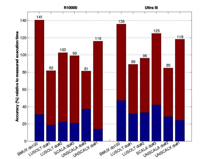
• Provide the compiler with information to
  enable performance related optimizations
• Predict the execution time of scientific
  Fortran programs, with reasonable
  accuracy, using architecture independent
  models
• Rapid performance tuning tool
• Architecture evaluation
• Fast performance estimation results with
  reasonable accuracy
  – light load on the compiler
  – rapid feedback to the user
• Abstract models (symbolic expressions), as
  a function of
  – program constructs
  – input data set
  – architecture parameters
• Model different parts of the system
  independently
• Each model generates one or more terms in
  a symbolic expression
• Advantages
  – simplicity
  – modularity
  – extensibility
You can also read