Deep Learning Based Rib Centerline Extraction and Labeling
←
→
Page content transcription
If your browser does not render page correctly, please read the page content below
Deep Learning Based Rib Centerline Extraction
                                                         and Labeling

                                                 Matthias Lenga, Tobias Klinder, Christian Bürger, Jens von Berg,
                                                                  Astrid Franz, Cristian Lorenz

                                                              Philips Research Europe, Hamburg, Germany
arXiv:1809.07082v2 [cs.CV] 14 Jan 2019

                                                 Abstract. Automated extraction and labeling of rib centerlines is a
                                                 typically needed prerequisite for more advanced assisted reading tools
                                                 that help the radiologist to efficiently inspect all 24 ribs in a CT vol-
                                                 ume. In this paper, we combine a deep learning-based rib detection with
                                                 a dedicated centerline extraction algorithm applied to the detection re-
                                                 sult for the purpose of fast, robust and accurate rib centerline extraction
                                                 and labeling from CT volumes. More specifically, we first apply a fully
                                                 convolutional neural network (FCNN) to generate a probability map for
                                                 detecting the first rib pair, the twelfth rib pair, and the collection of all
                                                 intermediate ribs. In a second stage, a newly designed centerline extrac-
                                                 tion algorithm is applied to this multi-label probability map. Finally,
                                                 the distinct detection of first and twelfth rib separately, allows to de-
                                                 rive individual rib labels by simple sorting and counting the detected
                                                 centerlines. We applied our method to CT volumes from 116 patients
                                                 which included a variety of different challenges and achieved a centerline
                                                 accuracy of 0.787 mm with respect to manual centerline annotations.

                                                 Keywords: Rib segmentation, deep learning, fully convolutional neural
                                                 networks, whole-body CT scans, trauma.

                                         1     Introduction
                                         The reading of the ribs from 3D CT scans is a typical task in radiology, e.g., to
                                         find bone lesions or identify fractures. During reading, each of the 24 ribs needs
                                         to be followed individually while scrolling through the slices. As a result, this
                                         task is time-consuming and rib abnormalities are likely to be overlooked.
                                             In order to assist reading, efficient visualization schemes or methods for nav-
                                         igation support are required. These applications are typically based on the rib
                                         centerlines, cf. [7,8]. Despite their generally high contrast, automated extraction
                                         of the rib centerlines from CT is challenging. For example, image noise and ar-
                                         tifacts impede the extraction, but also other bony structures in close vicinity
                                         (most prominently the vertebra), as well as severe pathologies. Finally, anatom-
                                         ical labeling of the extracted centerlines (i.e. knowing which one for example is
                                             This is a preprint version of [1]. The final authenticated publication is available
                                             online at https://doi.org/10.1007/978-3-030-11166-3 9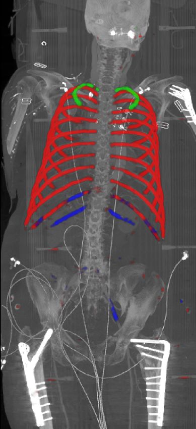
2

the “7th right rib”) is usually desirable. From an algorithmic perspective, this
task is trivial if all 24 ribs are correctly extracted, as simply counting left and
right ribs from cranial to caudal would be sufficient. Obviously, this task becomes
significantly more challenging once the rib cage is only partially imaged or once
a rib is missing (e.g., due to pathologies or missed detection in a previous step).
    A wide range of different approaches has been proposed in the past for rib
centerline extraction partially also including their labeling. Tracing based ap-
proaches, as in [4,6] aim at iteratively following the ribs. As such approaches
rely on an initial seed point detection per rib, an entire rib is easily missed once
a corresponding seed point was not detected. Alternatively, potential rib candi-
dates can be first detected in the entire volume which then need to be grouped
to obtain ribs, as for example done in [5]. However, the removal of other falsely
detected structures remains a crucial task. Attempts have been made to addi-
tionally integrate prior knowledge by means of geometrical rib cage centerline
models, cf. [3,8]. Nevertheless, such approaches may struggle with deviations
from the model in terms of pathologies.
    In this paper, we propose a two-stage approach combining deep learning and
classic image processing techniques to overcome several of the limitations listed
above. Rib probability maps are calculated at first using a fully convolutional
neural network, see Subsection 2.2, and then the centerlines are reconstructed
using a specifically designed centerline extraction algorithm as described in Sub-
section 2.3. In particular, three distinct rib probability maps are calculated (first
rib, twelfth rib or intermediate rib). By knowing the first and/or twelfth rib, la-
beling can be solved easily by iterative counting. This scheme also works in
case of partial rib cages (for example if only the upper or lower part is shown).
Evaluation is carried out on a representative number of 116 cases.

2     Methods

2.1   Data

Our data set consists in total of 116 image volumes containing 62 thorax as well
as 54 full body CT scans. The data includes a wide range of typical challenges,
such as variation in the field of view leading to partly visible or missing ribs (3
patients with first rib missing, 38 patients with at least partially missing twelfth
rib), various types of rib fractures, spine scoliosis (14 patients) strong contrast-
uptake around the first rib (33 patients), implants in other bony structures (7
around the sternum, 2 around the spine, and 2 around the femur/humerus),
several different devices with similar intensity to the ribs such as catheters or
cables (57 patients).
    In each image, we annotated rib centerlines by manually placing spline control
points. The rib centerlines were then obtained using cubic spline interpolation.
For each image volume, we generated a label mask by dilating the corresponding
centerlines with a radius of 3.0 mm. Four different labels are assigned to the
classes background, first rib, twelfth rib and intermediate rib.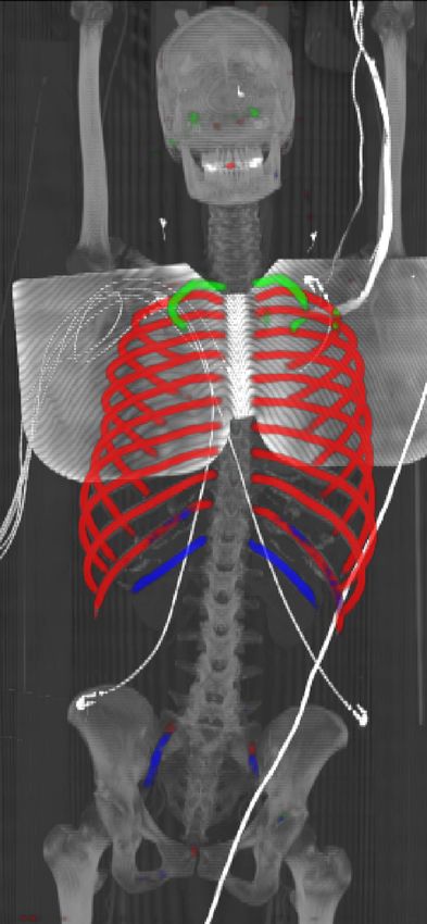
Deep Learning Based Rib Centerline Extraction and Labeling              3

2.2   Multi-Label Rib Probability Map Generation

For rib detection, we first apply a fully convolutional neural network (FCNN) in
order to generate probability maps which are subsequently fed into the tracing
algorithm described in Subsection 2.3. More specifically, we formulate our task
as a 4-class problem, where the network yields for each voxel vijk of the volume a
4-dimensional vector pijk ∈ [0, 1]4 . The components pijk,0 , pijk,1 , pijk,2 , pijk,3 can
be interpreted as probabilities that the associated voxel belongs to the classes
background, first rib (pair), twelfth rib (pair) or intermediate rib (pairs), respec-
tively. Distinct classes for the first and the twelfth rib were introduced to deal
with differences in anatomy (especially for the first rib) while significantly sim-
plifying the following labelling procedure. By using the relative to location of
the intermediate ribs to the first and twelfth rib, labelling of the ribs can be
achieved efficiently. Moreover, knowing the potential location of first or twelfth
rib enables labelling even in cases of partial rib cages. Details are provided in
Subsection 2.3 below.
     We favored the parsimonious 4-class learning task over training a neural
network for detecting each individual rib, resulting in a 25-class (24 ribs plus
background) classification problem, due to several reasons: i) The 4-class network
in combination with our iterative tracing approach seems sufficient for solving
the problem at hand, ii) due to the similar appearance of intermediate ribs, we
do not expect the 25-class network to be able to identify internal ribs reliably,
iii) the 25-class approach would cause a higher memory footprint and runtime
during training and inference.
     As network architecture, we chose the Foveal network described in [2]. Ba-
sically, the network is composed of two different types of layer modules, CBR
and CBRU blocks, see Figure 1. A CBR block consists of a 3 × 3 × 3 valid
convolution (C) followed by batch normalization (B) and a rectified linear unit
activation (R). A CBRU block is a CBR block followed by an average unpool-
ing layer (U). Since we favor fast network execution times and a moderate GPU
memory consumption, we decided to use three resolution layers LH , LM , LL , each
composed of three CBR blocks. Differently sized image patches with different
isotropic voxel spacings are fed into the layers as input, see Table 1. The low and
medium resolution pathways LL , LM are integrated into the high resolution layer
LH using CBRU blocks. Implementation details and further remarks concerning
the architecture performance can be found in [2].

                               input patch size (voxel) patch voxel spacing (mm)
      LH original resolution        66 × 66 × 66             1.5 × 1.5 × 1.5
      LM medium resolution          38 × 38 × 38             3.0 × 3.0 × 3.0
        LL low resolution           24 × 24 × 24             6.0 × 6.0 × 6.0

                 Table 1. Input configuration of the network layers.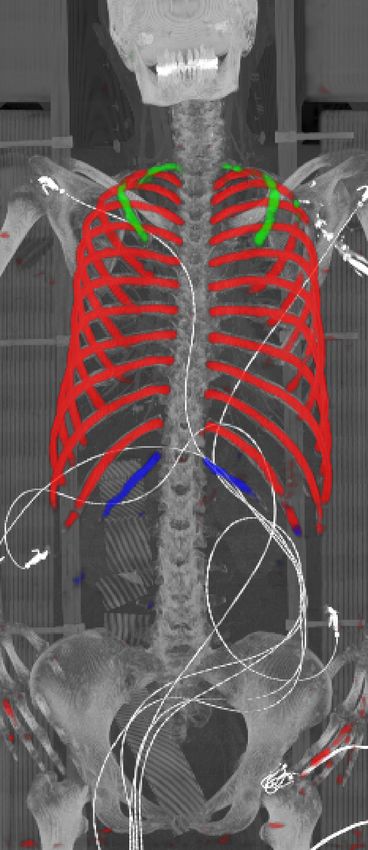
4

    As preprocessing, the CT images are resampled to an isotropic spacing of 1.5
mm using linear interpolation and normalized to zero mean and unit standard
deviation. The network was trained by minimizing the cross entropy on mini-
batches containing 8 patches (each at three different resolutions) drawn from
8 randomly selected images. In order to compensate for the class imbalance
between background and rib voxels, we used the following randomized sampling
strategy: 10% of the patch centers were sampled from the bounding box of the
first rib pair, 10% from the bounding box of the twelfth rib pair and 30% from the
bounding box of the intermediate ribs. The remaining 50% patch centers were
uniformly sampled from the entire volume. As an update rule, we chose AdaDelta
[9] in combination with a learning rate schedule. For data augmentation, the
patches were randomly scaled and rotated around all three axes. The neural
network was implemented with CNTK version 2.2 and trained for 2000 epochs
on a GeForce GTX 1080. The network training could be completed within a
few hours and network inference times were ranging from approximately 5 to 20
seconds, depending on the size of the input CT volume.

2.3   Centerline Extraction and Labeling
In order to robustly obtain rib centerlines, we designed an algorithm that specif-
ically incorporates the available information from the multi-label probability
map. It basically consists of four distinct steps:
 1. Determination of a rib cage bounding box.
 2. Detection of an initial left and right rib.
 3. Tracing of the detected ribs and detecting neighboring ribs iteratively up-
    wards and downwards of the traced rib.
 4. Rib labeling.
Steps 1 to 3 are performed on the combined probability map, adding the results of
the three non-background classes and limiting the sum to a total probability of
1.0, i.e. to each voxel vijk we assign the value qijk := min{pijk,1 +pijk,2 +pijk,3 , 1}.

Step 1: Bounding Box Detection
Generally, the given CT volume is assumed to cover at least a large portion of
the rib cage, but may extend beyond it. Therefore, we first determine a search
region in order to identify the visible ribs. Based on the axial image slices, a
2D bounding rectangle is computed using a probability threshold of 0.5 on the
combined probability map. To suppress spurious responses, we require a minimal
2D box size of 30 mm×10 mm to be a valid bounding box. From the set of valid
2D bounding boxes, a 3D bounding box is calculated from the largest connected
stack in vertical direction. The 3D bounding box is strictly speaking not a box,
but has inclined faces. Each of the 4 faces results from a linear regression of the
slice wise determined 4 border positions, having the advantage of being robust
against outliers and being able to represent to some extent the narrowing of the
rib cage from abdomen to shoulders (see Figure 2 a,b).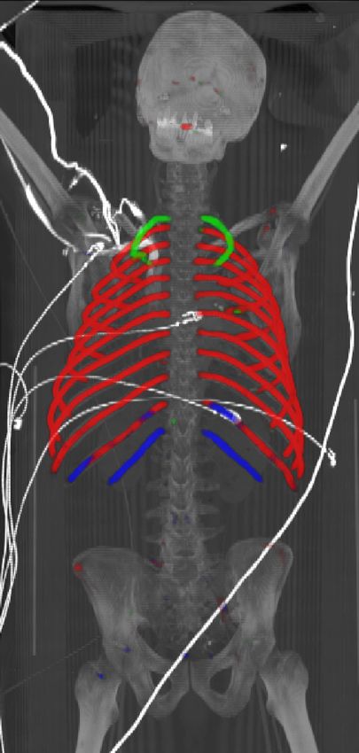
Deep Learning Based Rib Centerline Extraction and Labeling 5
Fig. 1. Foveal architecture with 3 resolution levels. The feature extraction pathways
(green), consisting of 3 CBR blocks, are integrated using CBRU blocks (blue). The
final CS block consists of a 3 × 3 × 3 valid convolution and a soft-max layer.
(a) (b) (c)
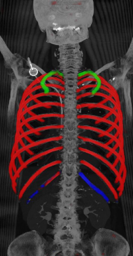
Fig. 2. (a) Neural network output (green: first rib; red: intermediate rib; blue: twelfth
rib) and approximate 3D bounding box of the rib cage (yellow) in coronal (top) and
axial view (bottom). The lower image depicts in light blue the two search regions for
rib detection. (b) Schematic representation of the vertical stack of 2D bounding boxes
(red) in coronal view and the approximate 3D bounding box of the rib cage resulting
from the largest connected stack in vertical direction by linear regression (yellow). The
dashed yellow line marks the box section at medium axial level. The two search regions
used for initial rib detection are depicted in light blue. (c) Traced ribs (red) are shown
on top of a sagittal cross-section of the probability map. The fan-like search regions
for neighboring ribs are depicted in yellow.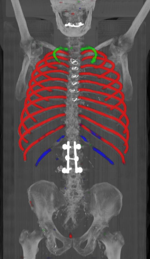
6

Step 2: Initial Rib Detection
From the approximate rib cage bounding box obtained in Step 1, we derive an
initial cross-sectional search window to detect the ribs. For that purpose, anchor
point al , ar are chosen at 25% and 75% of the left-to-right extension of the box
section at medium axial level. Then sagittal 2D search regions centered at al
and ar of spacial extension 100 mm× 100 mm are defined (see Figure 2 a,b). In
each of these regions an initialization point exceeding a probability of 0.5 is de-
termined. We remark that this point may be located at the rib border. To locate
the rib center, we sample the probability values in a spherical region of 15 mm
diameter around the initialization point. Next, the probability weighted center
of mass c0 ∈ R3 and the probability weighted covariance matrix Σ0 ∈ R3×3 of
the voxel coordinates are calculated. Finally, we use c0 as rib center estimate
and the eigenvector t0 ∈ R3 corresponding to the largest eigenvalue of Σ0 as
estimation of the tangential direction. The position c0 is added to the list of rib
center line control points.

Step 3: Rib Tracing and Detection of Neighboring Ribs
Based on the initial rib detection result from Step 2, the rib response in the
probability map is traced in an iterated scheme (i = 0, 1, 2...) consisting of the
following three actions:
a) Starting from ci move in tangential direction ti until a voxel with combined
   probability value qijk < 0.5 is encountered or a maximal moving distance of
   7.5 mm is reached.
b) Calculate the weighted mean vector ci+1 ∈ R3 in a spherical region around
   the current position. Add ci+1 to the list of rib center line control points and
   move to ci+1 .
c) Calculate the probability weighted covariance matrix Σi+1 ∈ R3×3 in a
   spherical region around ci+1 and compute the tangential direction ti+1 ∈ R3 ,
   see Step 2.
    This scheme is iterated until the moving distance in the current iteration
falls below a predefined threshold of 3.0 mm. In that case, a forward-looking
mechanism is triggered which aims at bridging local drop-outs of the probability
response. More precisely, the algorithm searches for a voxel with a combined
probability value exceeding 0.5 within a cone-shaped region. This voxel then
serves as continuation point for the iterative tracing procedure described above.
    Tracing from the initial starting point c0 is performed in both possible di-
rections and results are finally concatenated which yields a centerline of the full
rib represented by the point sequence {c0 , c1 , ...}. After the tracing of one rib is
completed, the resulting centerline is inserted into the list of rib centerlines L
which is ordered in vertical direction from feet to head.
    This collection is extended in a step wise fashion by detecting adjacent so
far untraced ribs using fan-like 2D search regions anchored at the lowest and
highest rib contained in L (see Figure 2b).
    The initial location of the search fan is 10 mm distal from the rib starting
point at the spine. The rib tangential vector at this point is used as normal vec-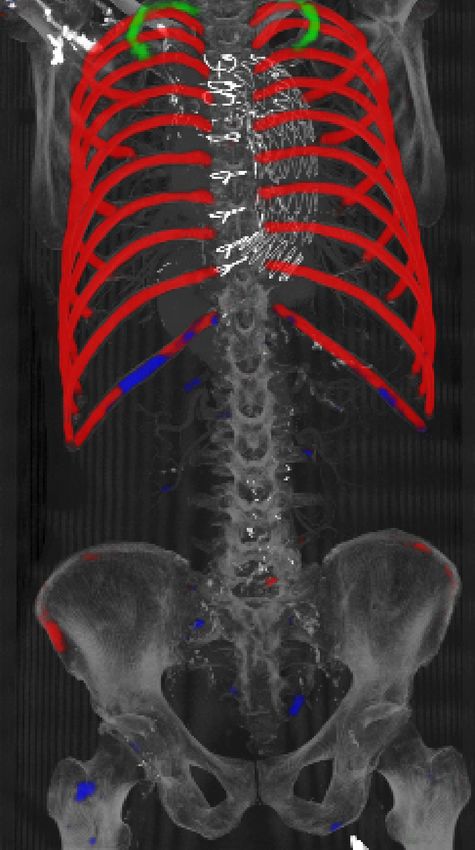
Deep Learning Based Rib Centerline Extraction and Labeling          7

Fig. 3. Schematic representation of the iterative tracing algorithm. Each red point
corresponds to a probability weighted mean vector ci in the spherical region around
the associated preceding position which depicted by a yellow point connected by a
yellow arrow (see Step 3b). The black arrows correspond to a movement in tangential
direction ti (see Step 3a). The blue triangle depicts the cone-shaped search region
used by the forward-looking mechanism. The rib center line resulting from a spline
interpolation of the control points ci is depicted by the dashed red line.

tor of the fan plane. The fan opening direction withing this plane is steered by
the intersection point of the previous rib with the fan plane. If only one traced
rib is available yet, the fan is simply pointing upward or downward. If a neigh-
boring rib could be found within the fan, the iterative scheme described above
is applied to trace the rib. If not, the search fan is moved along the rib in 10 mm
steps towards the distal end.

Step 4: Rib Labeling
After extraction of the centerlines, the average probability for all three non-
background classes is calculated for each found rib. In the optimal case, 12 rib
pairs have been found and the first and twelfth rib have an average probability
along their centerlines above 0.5 for their respective class. In this case, the in-
termediate ribs are labeled according to their position in the list L. In case that
less than 12 ribs were traced, the labeling is still possible if either the first or
twelfth rib can be identified. Labeling is not possible if both first and twelfth rib
cannot be identified and less then 10 ribs were traced.

3   Results

Our pipeline was evaluated using 4-fold cross validation (CV). More precisely, the
dataset was randomly shuffled and partitioned into 4 equally sized subsamples
each containing 29 images. We trained 4 different networks by using in each fold
three subsamples as training data while retaining a single subsample as validation
data for testing. In this way, it is ensure that each data set was contained once
in a testing subsample and as a result one probability map was obtained per
case.
8

3.1   Multi-Label Network
For the evaluation of a probability map pijk = (pijk,0 , pijk,1 , pijk,2 , pijk,3 ) gen-
erated by the neural network, we assigned to each voxel vijk a predicted class
label Lpred
       ijk based on its maximal class response, i.e.

                           Lpred
                            ijk = argmaxc=0,1,2,3 pijk,c .

Following the naming convention from Subsection 2.2, the labels 0, 1, 2, 3 corre-
spond to the classes background, first rib, twelfth rib and intermediate rib, re-
spectively. Comparing the predicted class labels with the corresponding ground
truth labels LGT
              ijk , yields for each class the number of true positives (TP), false
positives (FP), and false negatives (FN), i.e.
                                                pred
                    TPC = |{ijk : LGT
                                   ijk = C and Lijk = C}|
                                                 pred
                    FPC = |{ijk : LGT
                                   ijk 6= C and Lijk = C}|
                                                pred
                    FNC = |{ijk : LGT
                                   ijk = C and Lijk 6= C}|

where C ∈ {0, 1, 2, 3} denotes the class under consideration. Henceforth, we
will omit the class index C in order to simplify the notation. Based on these
quantities we compute for each class sensitivity, precision and Dice as follows:
                                           TP
                           sensitivity =
                                         TP + FN
                                           TP
                             precision =                                            (1)
                                         TP + FP
                                              2TP
                                 Dice =
                                         2TP + FP + FN
Table 2 displays the statistics of the aforementioned measures calculated on the
label images contained in the test sets from the 4-fold CV. For the class labels
first rib and intermediate rib all 116 images were considered. For the class label
twelfth rib we excluded 21 images from our evaluation which did not contain any
part of the twelfth rib pair.
     In order to analyze the overall rib detection rate irrespective of the specific
rib class, we assigned a single label to each non-background voxel. Based on these
combined masks, we again calculated the statistical measures from Equation 1
on all 116 images. The obtained results are summarized in Table 2 as class label
rib.
As can be seen from Table 2, we obtain overall good performance for the overall
rib detection captured for example with an mean Dice of 0.84. Let us remark that
for thin objects, such as the dilated rib centerlines, the Dice score constitutes
a rather sensitive measure. The results indicate that detecting the first and
twelfth rib pairs is more difficult for our network. While extraction of the first
rib is more challenging due to, e.g., higher noise in the upper thorax or other
bony structures in close vicinity (clavicle, shoulder blades, vertebrae), the twelfth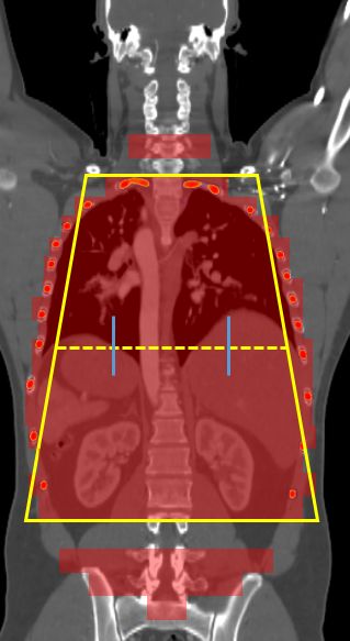
Deep Learning Based Rib Centerline Extraction and Labeling                   9

      first rib    sens.   prec.   Dice                   twelfth rib   sens.   prec.   Dice
        mean        0.65    0.70   0.67                      mean        0.60    0.63   0.59
         std.       0.13    0.12   0.12                      std.        0.22    0.23   0.20
      25% qrt.      0.58    0.66   0.62                    25% qrt.      0.49    0.54   0.47
       median       0.66    0.73   0.70                     median       0.66    0.71   0.64
      75% qrt.      0.74    0.78   0.74                    75% qrt.      0.77    0.81   0.74

intermediate rib sens. prec. Dice                             rib       sens.   prec.   Dice
      mean        0.81 0.87 0.84                             mean        0.81    0.87   0.84
      std.        0.07 0.04 0.05                             std.        0.07    0.04   0.05
    25% qrt.      0.79 0.84 0.82                           25% qrt.      0.79    0.84   0.82
     median       0.82 0.87 0.84                            median       0.82    0.87   0.84
    75% qrt.      0.85 0.90 0.87                           75% qrt.      0.84    0.90   0.86

Table 2. Mean, standard deviation, 25% quartile, median and 75% quartile of the
statistical measures for the predicted class labels first rib, intermediate rib, twelfth rib
and the combined class rib.

rib can be extremely short and is easily confused by the neighboring ribs. For
further illustration, Figure 4 shows the results on selected representative cases.
Generally, the ribs are well detected without major false responses in other
structures - despite all the different challenges present in the data. The color
coding highlighting of the multi-label detection reveals that first and twelfth are
mostly correctly detected. In few cases the network wrongly generated strong
responses of the classes first rib or last rib for voxels belonging to the second or
eleventh rib pair.

3.2     Rib centerlines
For the evaluation of the final centerlines, both ground truth lines and automat-
ically determined centerlines were resampled to 1.0 mm uniform point distance.
A true positive distance of δ = 5.0 mm was chosen such that, if for a ground
truth point (GTP) no result point within δ was found, the GTP was counted as
false negative (FN). Result points having a corresponding GTP within δ were
counted as true positive (TP), all other as false positive (FP). From the TP, FP,
and FN values we calculated sensitivity, precision and Dice using Equation (1).
    Table 3 summarizes our results from the 4-fold cross-validation. The point
wise responses (TP, FP, FN) are averaged up over all cases. The evaluation
measures are finally reported on a per rib basis, as well as for all ribs. The
Euclidean distance (dist.) is measured as point-to-line distance between result
point and ground truth line. Moreover, Table 4 contains the percentage of cases
with missed labeled ribs. Here, a rib is counted as missed, if less than half of the
ground truth rib centerline could be detected. A detected rib centerline point
counts only as true positive if the correct label was determined.
    With an average Euclidean distance error of 0.787 mm, we obtained an overall
result that is generally better compared to what is reported in the state of the art.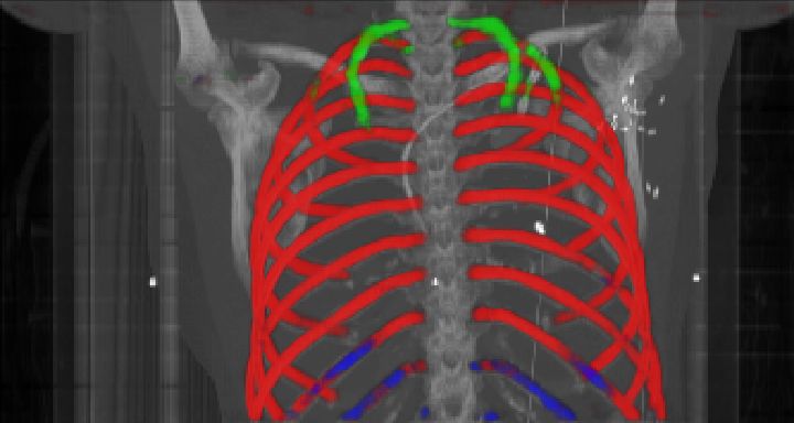
10

Although, it needs to be kept in mind that results are unfortunately not directly
comparable as both the data sets as well the evaluation metrics significantly differ
across prior work. Similarly to the results obtained on the probability maps,
distance errors are significantly higher for first and twelfth rib compared to the
rest of the rib cage. As discussed, this is caused by the intrinsic challenges of
these ribs, but certainly also an affect of error propagation in that sense that the
quality of the probability maps also impacts centerline extraction. Interestingly,
the right ribs are generally slightly worse compared to the left ribs, probably due
to a slightly unbalanced data set with more challenges on the right side. Figure
5 shows the centerlines which were automatically generated using our walker
algorithm from the corresponding network outputs displayed in Figure 4.

4    Conclusion

We presented a fully automated two-stage approach for rib centerline extraction
and labelling from CT images. First, multi-label probability maps (containing
the classes first rib, twelfth rib, intermediate ribs, background) are calculated
using a fully convolutional neural network and then centerlines are extracted
from this multi-label information using a tracing algorithm. For assessment,we
performed a 4-fold cross validation on a set of 116 cases which includes several
cases displaying typical clinical challenges. Comparing the automated extraction
results to our manual ground truth, we were able to achieve an Euclidean distance
error of 0.787 mm. The 4-class label detection was crucial to simplify rib labelling
by taking the network responses associated to the classes first rib and twelfth
rib into account. Compared to a distinct detection of first and twelfth rib using
separate networks, our multi-label task was chosen as it is memory and run-time
efficient with negligible loss in final centerline accuracy.
     In contrast to other approaches, no strong anatomical prior knowledge, e.g.,
in the form of geometrical models, was explicitly encoded into our pipeline to
deal with pathological deviations. Future work will focus on improving the per-
formance of the neural network by using motion field and registration based
data augmentation techniques and a more advanced data-driven image prepro-
cessing. Moreover, we are currently investigating further improvements of our
walker algorithm and the network architecture.

References
 1. M. Lenga, T. Klinder, C. Bürger, J. von Berg, A. Franz, C. Lorenz (2019) Deep
    Learning Based Rib Centerline Extraction and Labeling. In: Vrtovec T., Yao J.,
    Zheng G., Pozo J. (eds) Computational Methods and Clinical Applications in Mus-
    culoskeletal Imaging. MSKI 2018. Lecture Notes in Computer Science, vol 11404.
    Springer, Cham; https://doi.org/10.1007/978-3-030-11166-3 9
 2. T. Brosch and A. Saalbach, “Foveal fully convolutional nets for multi-organ seg-
    mentation”, Proc. SPIE Medical Imaging 2018: Image Processing, vol. 10574,
    105740U; https://doi.org/10.1117/12.2293528
Deep Learning Based Rib Centerline Extraction and Labeling 11
3. T. Klinder, C. Lorenz, J. von Berg, S. Dries, T. Bülow, J. Ostermann, “Automated
model-based rib cage segmentation and labeling in CT images”, In: Proc. MICCAI.
LNCS 4792 (2007), pp. 195-203
4. H. Shen, L. Liang, M. Shao, and S. Qing, “Tracing Based Segmentation for the La-
beling of Individual Rib Structures in Chest CT Volume Data” In: Proc. MICCAI,
LNCS 3217 (2004), pp. 967-974
5. J. Staal, B. van Ginneken, M. A. Viergever, “Automatic rib segmentation and
labeling in computed tomography scans using a general framework for detection,
recognition and segmentation of objects in volumetric data”, Medical Image Anal-
ysis 11 (2006), pp. 35-46
6. J. Lee and A. P. Reeves, “Segmentation of individual ribs from low dose chest CT”,
Proc. SPIE 2010: Computer aided Diagnosis, vol. 7624, pp. 76243J, 2010.
7. C. Tobon-Gomez, T. Stroud, J. Cameron, D. Elcock, A. Murray, D. Wyeth, C.
Conway, S. Reynolds, P. Augusto Gondim Teixeira, A. Blum, C. Plakas, “OpenRib
Clinical Application”, MSK Workshop 2017
8. D. Wu, D. Liu, Z. Puskas, C. Lu, A. Wimmer, C. Tietjen, G. Soza, S. Kevin Zhou,
“A Learning Based Deformable Template Matching Method for Automatic Rib
Centerline Extraction and Labeling in CT Images” CVPR, 2008
9. Zeiler, M. D., ADADELTA: an adaptive learning rate method, arXiv preprint
arXiv:1212.5701 (2012).
10. L. Zhang, X. Li, Q. Hu, Automatic Rib Segmentation in Chest CT Volume Data,
ISBI 201212
rib sens. prec. dist.(mm) Dice
01l 0.878 0.927 1.431 0.902
01r 0.871 0.915 1.511 0.894
02l 0.972 0.971 0.878 0.972
02r 0.952 0.963 0.880 0.957
03l 0.981 0.984 0.782 0.983
03r 0.976 0.973 0.854 0.975
04l 0.989 0.994 0.740 0.992
04r 0.984 0.984 0.785 0.984
05l 0.994 0.993 0.763 0.993
05r 0.972 0.978 0.811 0.975
06l 0.994 0.992 0.757 0.993
06r 0.964 0.965 0.757 0.964
07l 0.991 0.995 0.731 0.993
07r 0.969 0.957 0.721 0.963
08l 0.992 0.984 0.730 0.988
08r 0.969 0.968 0.719 0.969
09l 0.993 0.993 0.738 0.993
09r 0.973 0.971 0.699 0.972
10l 0.986 0.992 0.715 0.989
10r 0.965 0.969 0.674 0.967
11l 0.984 0.974 0.732 0.979
11r 0.961 0.962 0.665 0.962
12l 0.917 0.972 0.921 0.944
12r 0.886 0.942 0.905 0.914
all ribs 0.972 0.976 0.787 0.974
Table 3. Rib-wise evaluation of the method based on the final labeled centerline point
sets. A detected rib centerline point counts only as true positive if the correct label
was determined. The table shows the summary for the collected 116 cases and reports
sensitivity, precision, Euclidean distance and Dice score.
No. missed ribs Case percentage
0 81.6 %
1 8.8 %
2 7.0 %
≥3 2.6 %
Table 4. Percentage of cases with missed labeled ribs. A rib counts as missed, if less
than half of the ground truth rib centerline could be detected. A detected rib centerline
point counts only as true positive if the correct label was determined.Deep Learning Based Rib Centerline Extraction and Labeling 13
(a) (b) (c) (d)
(e) (f) (g) (h)
(i) (j)
Fig. 4. Maximum intensity projections (MIP) of selected CT volumes overlaid with the
multi-label output of the neural network (green: first rib; red: intermediate rib; blue:
twelfth rib). The selected case above display common difficulties which are inherent in
the data set, such as pads (a) or cables (b), internal devices such as pacemakers (c),
stents (d), spinal (e) and femural/humeral implants (f), injected contrast agents (g),
patient shape variations such as scoliosis (h), limited field of views (FOVs), i.e. partly
missing first (i) or twelfth rib (j).14
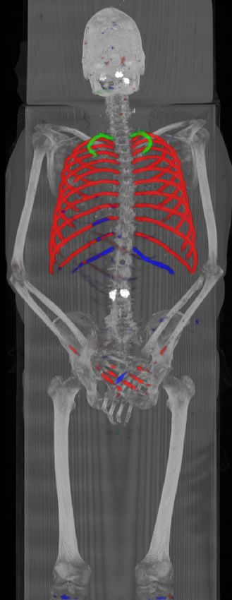
(a) (b) (c) (d)
(e) (f) (g) (h)
(i) (j)
Fig. 5. Automatically generated centerline splines associated with the FCNN outputs
displayed in Figure 4. The selected case above display common difficulties which are
inherent in the data set, such as pads (a) or cables (b), internal devices such as pace-
makers (c), stents (d), spinal (e) and femural/humeral implants (f), injected contrast
agents (g), patient shape variations such as scoliosis (h), limited field of views (FOVs),
i.e. partly missing first (i) or twelfth rib (j).You can also read