Description and evaluation of the UKCA stratosphere-troposphere chemistry scheme (StratTrop vn 1.0) implemented in UKESM1
←
→
Page content transcription
If your browser does not render page correctly, please read the page content below
Geosci. Model Dev., 13, 1223–1266, 2020
https://doi.org/10.5194/gmd-13-1223-2020
© Author(s) 2020. This work is distributed under
the Creative Commons Attribution 4.0 License.

Description and evaluation of the UKCA stratosphere–troposphere
chemistry scheme (StratTrop vn 1.0) implemented in UKESM1
Alexander T. Archibald1,2 , Fiona M. O’Connor3 , Nathan Luke Abraham1,2 , Scott Archer-Nicholls1 ,
Martyn P. Chipperfield4,5 , Mohit Dalvi3 , Gerd A. Folberth3 , Fraser Dennison6,a , Sandip S. Dhomse4,5 ,
Paul T. Griffiths1,2 , Catherine Hardacre3 , Alan J. Hewitt3 , Richard S. Hill3 , Colin E. Johnson3 , James Keeble1,2 ,
Marcus O. Köhler1,7,b , Olaf Morgenstern6 , Jane P. Mulcahy3 , Carlos Ordóñez3,c , Richard J. Pope4,5 ,
Steven T. Rumbold8 , Maria R. Russo1,2 , Nicholas H. Savage3 , Alistair Sellar3 , Marc Stringer8 , Steven T. Turnock3 ,
Oliver Wild9 , and Guang Zeng6
1 Department  of Chemistry, University of Cambridge, Cambridge, CB2 1EW, UK
2 NCAS-Climate,    University of Cambridge, CB2 1EW, UK
3 Met Office Hadley Centre, FitzRoy Road, Exeter, EX1 3PB, UK
4 School of Earth and Environment, University of Leeds, Leeds, LS2 9JT, UK
5 National Centre for Earth Observation (NCEO), University of Leeds, Leeds, UK
6 National Institute of Water & Atmospheric Research Ltd (NIWA), 301 Evans Bay Parade, Greta Point,

Wellington, New Zealand
7 Centre for Ocean and Atmospheric Sciences, School of Environmental Sciences, University of East Anglia, Norwich, UK
8 NCAS-Climate, Department of Meteorology, University of Reading, Reading, RG6 6BB, UK
9 Lancaster Environment Centre, Lancaster University, Lancaster, LA1 4YQ, UK
a now at: CSIRO Oceans and Atmosphere, Aspendale, Australia
b now at ECMWF, Reading, UK
c now at: Departamento de Física de la Tierra y Astrofísica, Facultad de Ciencias Físicas, Universidad Complutense de

Madrid, Madrid 28040, Spain

Correspondence: Alexander Archibald (ata27@cam.ac.uk)

Received: 30 August 2019 – Discussion started: 25 September 2019
Revised: 7 January 2020 – Accepted: 19 January 2020 – Published: 17 March 2020

Abstract. Here we present a description of the UKCA Strat-        host model; simulations with the same chemical mechanism
Trop chemical mechanism, which is used in the UKESM1              run in an earlier version of the MetUM host model show a
Earth system model for CMIP6. The StratTrop chemical              range of sensitivity to emissions that the current model does
mechanism is a merger of previously well-evaluated tropo-         not fall within.
spheric and stratospheric mechanisms, and we provide re-             Whilst the general model performance is suitable for use in
sults from a series of bespoke integrations to assess the over-   the UKESM1 CMIP6 integrations, we note some shortcom-
all performance of the model.                                     ings in the scheme that future targeted studies will address.
   We find that the StratTrop scheme performs well when
compared to a wide array of observations. The analysis we
present here focuses on key components of atmospheric com-
position, namely the performance of the model to simulate         1   Introduction
ozone in the stratosphere and troposphere and constituents
that are important for ozone in these regions. We find that the   The ability to model the composition of the atmosphere is
results obtained for tropospheric ozone and its budget terms      vital for a wide range of applications relevant to society at
from the use of the StratTrop mechanism are sensitive to the      large. Atmospheric composition modelling can broadly be
                                                                  subdivided into two sub-disciplines: (1) aerosol processes

Published by Copernicus Publications on behalf of the European Geosciences Union.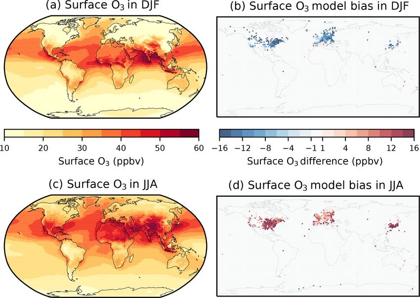
1224                                                                                  A. T. Archibald et al.: StratTrop vn 1.0

and microphysics and (2) atmospheric chemistry. Coupling          ine the effects on tropospheric oxidising capacity. Whilst the
these processes in climate models is paramount for being          chemical schemes described in O’Connor et al. (2014) (here-
able to simulate atmospheric composition at the global scale.     after OC14) and Morgenstern et al. (2009) (hereafter MO09)
The most societally important questions revolve around un-        have some overlap (for example the use of some common
derstanding how the composition of the atmosphere has             reactions) the schemes were developed with specific appli-
changed over the past, attributing this change, understand-       cations in scope. The reason for partitioning chemical com-
ing how this system is likely to change into the future, and      plexity like this is to reduce the computational resources re-
what the impacts of these changes are on the Earth system         quired. Moreover, simulations with these process limitations
and on human health. It is these pressing issues that have        were found to be able to capture the phenomena of interest.
led to the development of the new UK Earth system model,             However, increases in computational power and a drive to
UKESM1 (Sellar et al., 2019), which uses the UK Chem-             answer a greater number of questions from model simula-
istry and Aerosol model (UKCA) (O’Connor et al., 2014;            tions have allowed models that simulate both the stratosphere
Morgenstern et al., 2009; Mulcahy et al., 2018) as its key        and troposphere to be developed which are now widely used
component to simulate atmospheric composition in the Earth        (e.g. Pitari et al., 2002; Jöckel et al., 2006; Lamarque et al.,
system. The key challenge UKCA is applied to is under-            2008; Morgenstern et al., 2012). The removal of the need
standing and predicting how the concentrations of a range of      for prescribed upper boundary conditions (for the strato-
trace gases, especially the greenhouse gases methane (CH4 ),      sphere) and a more comprehensive chemistry scheme make
ozone (O3 ) and nitrous oxide (N2 O), and aerosol species will    their increased cost worth bearing. In this work, we de-
evolve in the Earth system under a range of different forcings.   scribe the implementation of a combined chemistry scheme
UKCA simulates the processes that control the formation and       suitable for simulating the stratosphere and the troposphere
destruction of these species. Here we describe and document       within the UKCA model as used in UKESM1 (Sellar et al.,
the performance of the version of UKCA used in UKESM1,            2019). This scheme, UKCA StratTrop, builds on and com-
which includes a representation of combined stratospheric         bines the existing stratospheric (MO09) and tropospheric
and tropospheric chemistry that enhances the capability of        schemes (OC14). In various configurations of UKCA (un-
UKCA beyond the version used in the Atmospheric Chem-             der the names HadGEM3-ES, UMUKCA-UCAM, NIWA-
istry and Climate Model Intercomparison Project (ACCMIP;          UKCA, ACCESS), this combined chemical scheme has al-
Young et al., 2013; O’Connor et al., 2014) and the recent         ready been used to study stratospheric ozone and its sensi-
Chemistry–Climate Model Initiative (CCMI) intercompari-           tivity to changes in bromine (Yang et al., 2014), subsequent
son (Bednarz et al., 2018; Hardiman et al., 2017; Morgen-         circulation changes (Braesicke et al., 2013) and how it may
stern et al., 2017). There have been a number of previous         be impacted by certain forms of geoengineering (Tang et
versions of UKCA with defined scopes, but we denote the           al., 2014); the role of ozone radiative feedback on temper-
version used in UKESM1 and described here as UKCA Strat-          ature and humidity biases at the tropical tropopause layer
Trop to signify its purpose of the holistic treatment of com-     (TTL) (Hardiman et al., 2015); the effects on tropospheric
position processes in the troposphere and stratosphere.           and stratospheric ozone changes under climate and emissions
   As a result of the Chemistry–Climate Model Validation          changes following the Representative Concentration Path-
Activity (CCMVal), it was recommended that models which           ways (RCPs) (Banerjee et al., 2016; Dhomse et al., 2018);
are aimed at simulating the coupled ozone–climate prob-           climate-induced changes in lightning (Banerjee et al., 2014);
lem should include processes to enable interactive ozone          and changes in methane chemistry between the present day
in the troposphere and stratosphere (Morgenstern et al.,          and the last interglacial (Quiquet et al., 2015). The scheme
2010). Chemistry–climate models (CCMs) use schemes to             has been included in model simulations as part of the CCMI
describe the reactions that chemical compounds undergo.           project (Eyring et al., 2013; Hardiman et al., 2017; Morgen-
These chemistry schemes can be constructed to explicitly          stern et al., 2017; Dhomse et al., 2018) as well as all future
model a specific chemical reaction system (e.g. Aumont et         Earth system modelling studies using the UKESM1 model
al., 2005), but in most applications the chemistry schemes        (Sellar et al., 2019).
are heavily simplified. Until recently, models of atmospheric        This paper is organised in the following sections: in
chemistry tended to focus on chemistry schemes formu-             Sect. 2, we present a thorough description of UKCA Strat-
lated for limited regions of the atmosphere; detailed schemes     Trop, including the physical model and details of the chem-
have been constructed to examine phenomena such as strato-        istry scheme, followed by a detailed description of the emis-
spheric ozone depletion or tropospheric air pollution. Exam-      sions used and some notes on the historical development of
ples of this using the UKCA model framework are two stud-         the scheme. In Sect. 3, we describe two 15-year simulations
ies of the effects of the eruption of Mt. Pinatubo, for which     we have performed with UKCA StratTrop in an atmosphere-
Telford et al. (2009) used the stratospheric scheme of Mor-       only configuration of UKESM1. In Sect. 4, we use these sim-
genstern et al. (2009) to study the effects of the eruption       ulations to review the performance of UKCA StratTrop, fo-
on stratospheric ozone, whereas Telford et al. (2010) used        cusing on the model’s ability to simulate key features of tro-
the tropospheric scheme of O’Connor et al. (2014) to exam-        pospheric and stratospheric chemistry as simulated by other

Geosci. Model Dev., 13, 1223–1266, 2020                                             www.geosci-model-dev.net/13/1223/2020/
A. T. Archibald et al.: StratTrop vn 1.0                                                                                      1225

models or observed using in situ and remote sensing mea-            downdrafts (Gregory and Allen, 1991), convective momen-
surements. Finally, in Sect. 5, we discuss the performance of       tum transport (Gregory et al., 1997) and convective available
the model and make some recommendations for further tar-            potential energy closure. The scheme involves diagnosis of
geted studies.                                                      possible convection from the boundary layer, followed by a
                                                                    call to shallow or deep convection on selected grid points
                                                                    based on the diagnosis from step one, and then a call to the
2     Model description                                             mid-level convection scheme at all points. One key difference
                                                                    between the convective treatment of UKCA chemical and
In this section, we present a thorough description of UKCA          aerosol tracers is that convective scavenging of aerosols (sim-
StratTrop, from the host physical model to the detailed pro-        ulated with GLOMAP-mode) is coupled with the convective
cess representation of the StratTrop chemistry scheme.              transport following Kipling et al. (2013), whereas for chem-
                                                                    ical tracers, convective transport and scavenging are treated
2.1    Physical model                                               independently. Further details on the convection scheme in
                                                                    GA7.1 can be found in Walters et al. (2019). Finally, mixing
The physical model to which the UKCA StratTrop chem-                over the full depth of the troposphere is carried out by the
istry scheme has been coupled is the Global Atmosphere              so-called “boundary layer” scheme in GA7.1; this scheme is
7.1/Global Land 7.0 (GA7.1/GL7.0; Walters et al., 2019)             that of Lock et al. (2000) but with updates from Lock (2001)
configuration of the Hadley Centre Global Environment               and Brown et al. (2008).
Model version 3 (HadGEM3; Hewitt et al., 2011).                        The GA7.1/GL7.0 configuration described in Walters et
   The coupling between the UKCA StratTrop chemistry                al. (2019) already includes the two-moment GLOMAP-mode
scheme and the GA7.1/GL7.0 configuration of HadGEM3 is              aerosol scheme from UKCA (Mann et al., 2010; Mulc-
based on the Met Office’s Unified Model (MetUM; Brown               ahy et al., 2018, 2020), in which sulfate and secondary or-
et al., 2012). As a result, UKCA uses aspects of Me-                ganic aerosol (SOA) formation is driven by prescribed oxi-
tUM for the large-scale advection, convective transport and         dant fields. In the UKCA–StratTrop configuration described
boundary layer mixing of its tracers. The large-scale advec-        here, the oxidants driving secondary aerosol formation are
tion makes use of the semi-implicit semi-Lagrangian for-            fully interactive; this coupling between UKCA chemistry and
mulation of the ENDGame dynamical core (Wood et al.,                GLOMAP-mode is fully described in Mulcahy et al. (2020).
2014) to solve the non-hydrostatic, fully compressible deep-        Together with dynamic vegetation and a terrestrial carbon
atmosphere equations of motion. These are discretised onto          and nitrogen scheme (Sellar et al., 2019), GA7.1/GL7.0 and
a regular latitude–longitude grid, with Arakawa C-grid stag-        UKCA StratTrop make up the atmospheric and land compo-
gering (Arakawa and Lamb, 1977). The discretisation in              nents of the UK Earth system model, UKESM1 (Sellar et al.,
the vertical uses Charney–Phillips staggering (Charney and          2019), which forms part of the UK contribution to the Sixth
Phillips, 1953) with terrain-following hybrid height coordi-        Coupled Model Intercomparison Project (CMIP6; Eyring et
nates. Although GA7.1/GL7.0 can be run at a variety of              al., 2016).
resolutions, as detailed in Walters et al. (2019), the reso-
lution here is N96L85 (1.875◦ × 1.25◦ longitude–latitude),          2.2   Chemistry scheme
i.e. approximately 135 km resolution in the horizontal and
with 85 terrain-following levels spanning the altitude range        The UKCA StratTrop scheme is based on a merger be-
from the surface to 85 km. Of the 85 model levels, 50 lie           tween the stratospheric scheme of MO09 and the tropo-
below 18 km and 35 levels are above 18 km (Walters et al.,          spheric “TropIsop” scheme of OC14. StratTrop simulates
2019). Mass conservation of UKCA tracers is achieved with           the Ox , HOx and NOx chemical cycles and the oxidation
the optimised conservative filter (OCF) scheme (Zerroukat           of carbon monoxide, ethane, propane, and isoprene in ad-
and Allen, 2015); use of this scheme for virtual dry potential      dition to chlorine and bromine chemistry, including hetero-
temperature resulted in reducing the warm bias at the TTL           geneous processes on polar stratospheric clouds (PSCs) and
(Hardiman et al., 2015; Walters et al., 2019). This conser-         liquid sulfate aerosols (SAs). The level of detail of the VOC
vation scheme is also used for moist prognostics (e.g. water        oxidation is far from the complexity of explicit representa-
vapour mass mixing ratio and prognostic cloud fields). Al-          tions (e.g. Aumont et al., 2005), but the VOCs simulated are
though this makes the conservation scheme for moist prog-           treated as discrete species.
nostics consistent with the treatment of UKCA tracers and              Wet deposition is parameterised using the approach of Gi-
virtual dry potential temperature, Walters et al. (2019) found      annakopoulos et al. (1999). Dry deposition is parameterised
that it had little impact on moisture biases in the lower strato-   employing a resistance type model (Wesely, 1989) using the
sphere.                                                             implementation described in OC14, updated to account for
   The convective transport of UKCA tracers is treated within       advancements in the Joint UK Land Environment Simulator
the MetUM convection scheme. It is essentially the mass flux        (JULES; Best et al., 2011), in particular a significant increase
scheme of Gregory and Rowntree (1990) but with updates for          in land surface types (an increase from 9 to 27; see below for

www.geosci-model-dev.net/13/1223/2020/                                                Geosci. Model Dev., 13, 1223–1266, 2020
1226                                                                                       A. T. Archibald et al.: StratTrop vn 1.0

more details). Interactive photolysis is represented with the      abundance of nitric acid trihydrate (NAT) and mixed NAT–
Fast-JX scheme (Neu et al., 2007), as implemented in Telford       ice polar stratospheric clouds is calculated following Chip-
et al. (2013). Fast-JX covers the wavelength range of 177 to       perfield (1999) assuming thermodynamic equilibrium with
750 nm. For shorter wavelengths, effective above 60 km of          gas-phase HNO3 and water vapour; the treatment of reactions
altitude, a correction is applied to the photolysis rates fol-     on liquid sulfate aerosol also follows Chipperfield (1999).
lowing the formulation of Lary and Pyle (1991).                    Sedimentation of PSCs is included in the model, whilst dehy-
   The StratTrop scheme includes emissions of 12 chemi-            dration is handled as part of the model’s hydrological cycle.
cal species: nitrogen oxide (NO), carbon monoxide (CO),            Denitrification is prescribed in the same way as in Chipper-
formaldehyde (HCHO), ethane (C2 H6 ), propane (C3 H8 ),            field (1999) with two different sedimentation velocities. We
acetaldehyde (CH3 CHO), acetone ((CH3 )2 CO), methanol             refer the reader to Morgenstern et al. (2009) and Dennison et
(CH3 OH) and isoprene (C5 H8 ) in addition to trace-gas            al. (2019) for further details.
aerosol precursor emissions (dimethyl sulfide (DMS), sulfur           The stratospheric sulfate aerosol optical depth, used in
dioxide (SO2 ) and monoterpenes). For the implementation           the radiation scheme of MetUM, is modified to be consis-
used in UKESM1, emissions may be prescribed or interactive         tent with the aerosols used in the heterogeneous chemistry
and are described in more detail in Sect. 2.6.1 to 2.6.3. A fur-   which, by default, are taken from a surface area density cli-
ther seven long-lived species (N2 O, CF2 Cl2 , CFCl3 , CH3 Br,     matology prepared for the CMIP6 model intercomparison
COS, H2 and CH4 ) are constrained by lower boundary con-           (Beiping Luo, personal communication, 2016). The surface
ditions; for more details see Sect. 2.6.4.                         aerosol density is converted to a mass mixing ratio using a
   UKCA StratTrop was developed by starting with the               climatology of particle size (Thomason and Peter, 2006) and
stratospheric chemistry scheme (MO09) and adding aspects           assuming a density of 1700 kg m−3 .
of chemistry unique to the tropospheric scheme (OC14). In
most cases the formulation and reaction coefficients are taken     2.3    Photolysis
from reference evaluations (JPL and IUPAC) or the Master
Chemical Mechanism, as detailed in OC14. Table 1 provides          The most significant new development relative to MO09 and
a list of the chemical tracers included in the StratTrop con-      OC14 in the UKCA–StratTrop scheme used in UKESM1 is
figuration used in UKESM1. In total the model employs 84           the interactive Fast-JX photolysis scheme, which is applied
species and represents the chemistry of 81 of these. O2 , N2       to derive photolysis rates between 177 and 750 nm (Neu et
and CO2 are not treated as chemically active species. Note         al., 2007) as described in Telford et al. (2013). This is an
that the scheme has a simplified treatment of stratospheric        important new addition as it enables interactive treatment of
halocarbons and lumps all chlorine and bromine source gases        photolysis rates (key drivers for the photochemistry of the at-
into CFC-11, CFC-12 and CH3 Br. This chemistry scheme              mosphere) under changing climate and atmospheric compo-
accounts for 199 bimolecular reactions (Table S1), 25 uni-         sition. For shorter wavelengths relevant above 60 km, a cor-
molecular and termolecular reactions (Table S2), 59 pho-           rection is added to account for photolysis occurring between
tolytic reactions (Table S3), 5 heterogeneous reactions (Ta-       112 and 177 nm, following Lary and Pyle (1991).
ble S4) and 3 aqueous-phase reactions for the sulfur cycle            In older versions of UKCA (i.e. MO09 and OC14) pre-
(Table S5). Hence, UKCA–StratTrop describes the oxidation          calculated photolysis frequencies were applied in the model.
of organic compounds – e.g. methane, ethane, propane and           Sellar et al. (2019) show a comparison of these and we note
isoprene and their oxidation products – coupled to the inor-       here that the switch from precalculated to online interactive
ganic chemistry of Ox , NOx , HOx , ClOx and BrOx using            photolysis calculations has had a significant effect on short-
a continuous set of equations with no artificial boundaries        ening the model-simulated methane lifetime and increasing
imposed on where to stop performing chemistry. Except for          the tropospheric mean [OH] (Telford et al., 2013; O’Connor
water vapour, at the top two levels, the mixing ratios of all      et al., 2014; Voulgarakis et al., 2009), as shown in Fig. 4.
species are held identical to those at the third-highest level.    2.4    Dry deposition
The time-dependent chemical reactions are integrated for-
ward in time using an implicit backward Euler solver with          In UKCA the representation of dry deposition follows the
Newton–Raphson iteration (Wild and Prather, 2000). This            resistance-in-series model as described by Wesely (1989) in
solver has a relative convergence criterion of 10−4 with a         which the removal of material at the surface is described by
time step of 60 min throughout the atmosphere. An extensive        three resistances: ra , rb and rc . The deposition velocity vd
discussion of the solver used here is presented in Esentürk et     (m s−1 ) is then a function of these three resistance terms ac-
al. (2018).                                                        cording to
   The treatment of polar stratospheric cloud (PSC) has been
                                                                               1
recently expanded in UKCA (Dennison et al., 2019), but             vd =                ,                                        (1)
these improvements did not make it into the UKESM1 ver-                   ra + rb + rc
sion of UKCA discussed here, which remains unmodified              where ra denotes the aerodynamic resistance to dry deposi-
from the original Morgenstern et al. (2009) scheme. The            tion, rb is the quasi-laminar resistance term and rc represents

Geosci. Model Dev., 13, 1223–1266, 2020                                                www.geosci-model-dev.net/13/1223/2020/
A. T. Archibald et al.: StratTrop vn 1.0                                                                                          1227

Table 1. List of chemical species in UKCA StratTrop. Species in italics are not advected tracers but are calculated using a steady-state
approximation. Species in bold are set as constant mixing ratios throughout the atmosphere.

                     Name                Formula                Dry deposited    Wet deposited    Emitted or LBC
                     O(3P)               O(3 P)                 No               No               No
                     O(1D)               O(1 D)                 No               No               No
                     O3                  O3                     Yes              No               No
                     N                   N                      No               No               No
                     NO                  NO                     Yes              No               Emitted
                     NO3                 NO3                    Yes              Yes              No
                     NO2                 NO2                    Yes              No               No
                     N2O5                N 2 O5                 Yes              Yes              No
                     HO2NO2              HO2 NO2                Yes              Yes              No
                     HONO2               HONO2                  Yes              Yes              No
                     H2O2                H 2 O2                 Yes              Yes              No
                     CH4                 CH4                    No               No               LBC
                     CO                  CO                     Yes              No               Emitted
                     HCHO                HCHO                   Yes              Yes              Emitted
                     MeOO                CH3 OO                 No               Yes              No
                     MeOOH               CH3 OOH                Yes              Yes              No
                     H                   H                      No               No               No
                     H2O                 H2 O                   No               No               No
                     OH                  OH                     No               No               No
                     HO2                 HO2                    No               Yes              No
                     Cl                  Cl                     No               No               No
                     Cl2O2               Cl2 O2                 No               No               No
                     ClO                 ClO                    No               No               No
                     OClO                OClO                   No               No               No
                     Br                  Br                     No               No               No
                     BrO                 BrO                    No               No               No
                     BrCl                BrCl                   No               No               No
                     BrONO2              BrONO2                 No               Yes              No
                     N2O                 N2 O                   No               No               LBC
                     HCl                 HCl                    Yes              Yes              No
                     HOCl                HOCl                   Yes              Yes              No
                     HBr                 HBr                    Yes              Yes              No
                     HOBr                HOBr                   Yes              Yes              No
                     ClONO2              ClONO2                 No               Yes              No
                     CFCl3               CFCl3                  No               No               LBC
                     CF2Cl2              CF2 Cl2                No               No               LBC
                     MeBr                CH3 Br                 No               No               LBC
                     HONO                HONO                   Yes              Yes              No
                     C2H6                C 2 H6                 No               No               Emitted
                     EtOO                C2 H5 OO               No               No               No
                     EtOOH               C2 H5 OOH              Yes              Yes              No
                     MeCHO               CH3 CHO                Yes              No               Emitted
                     MeCO3               CH3 C(O)OO             No               No               No
                     PAN                 PAN                    Yes              No               No
                     C3H8                C 3 H8                 No               No               Emitted
                     n-PrOO              C3 H7 OO               No               No               No
                     i-PrOO              CH3 CH(OO)CH3          No               No               No
                     n-PrOOH             C3 H7 OOH              Yes              Yes              No
                     i-PrOOH             CH3 CH(OOH)CH3         Yes              Yes              No
                     EtCHO               C2 H5 CHO              Yes              No               No
                     EtCO3               C2 H5 C(O)OO           No               No               No
                     Me2CO               CH3 C(O)CH3            No               No               Emitted
                     MeCOCH2OO           CH3 C(O)CH2 OO         No               No               No
                     MeCOCH2OOH          CH3 C(O)CH2 OOH        Yes              Yes              No

www.geosci-model-dev.net/13/1223/2020/                                                   Geosci. Model Dev., 13, 1223–1266, 2020
1228                                                                                                     A. T. Archibald et al.: StratTrop vn 1.0

Table 1. Continued.

                             Name                Formula                    Dry deposited   Wet deposited    Emitted or LBC
                             PPAN                PPAN                       Yes             No               No
                             MeONO2              MeONO2                     No              No               No
                             C5H8                C 5 H8                     No              No               Emitted
                             ISO2                HOC5 H8 OO                 No              No               No
                             ISOOH               HOC5 H8 OOH                Yes             Yes              No
                             ISON                ISON                       Yes             Yes              No
                             MACR                C 4 H6 O                   Yes             No               No
                             MACRO2              C4 H6 O(OO)                No              No               No
                             MACROOH             C4 H6 O(OOH)               Yes             Yes              No
                             MPAN                MPAN                       Yes             No               No
                             HACET               CH3 C(O)CH2 OH             Yes             Yes              No
                             MGLY                CH3 COCHHO                 Yes             Yes              No
                             NALD                NALD                       Yes             No               No
                             HCOOH               HC(O)OH                    Yes             Yes              No
                             MeCO3H              CH3 C(O)OOH                Yes             Yes              No
                             MeCO2H              CH3 C(O)OH                 Yes             Yes              No
                             H2                  H2                         No              No               LBC
                             MeOH                CH3 OH                     Yes             Yes              Emitted
                             CO2                 CO2                        No              No               No
                             O2                  O2                         No              No               No
                             N2                  N2                         No              No               No
                             DMS                 CH3 SCH3                   No              No               Emitted
                             SO2                 SO2                        Yes             Yes              Emitted
                             H2SO4               H2 SO4                     Yes             No               No
                             MSA                 MSA                        No              No               No
                             DMSO                DMSO                       Yes             Yes              No
                             COS                 COS                        No              No               Emitted
                             SO3                 SO3                        No              No               No
                             Monoterp            C10 H16                    Yes             No               Emitted
                             Sec_Org             ∗ Sec_Org                  Yes             Yes              No
                           ∗ The molecular mass of Sec_Org is set to 150 g mol−1 .

the resistance to uptake at the surface. Of these three terms rc                        The quasi-laminar resistance rb , on the other hand, de-
tends to be the most complex because it encompasses a vari-                          pends on the chemical and physical properties of the de-
ety of exchange fluxes, such as stomatal and cuticular uptake                        posited species. It describes the transport through the thin,
and assimilation by soil microbes. The uptake at the surface                         laminar layer of air closest to the surface. Transport through
also depends strongly on the presence of dew, rain or snow,                          this layer is diffusive due to the absence of turbulent mixing.
which can interrupt the deposition process altogether.                                  The third resistance term rc depends on both the physico-
   Surface dry deposition is calculated interactively at every                       chemical properties of the deposited species and the proper-
time step for a number of atmospheric gas-phase species (see                         ties and condition of the respective surface to which depo-
Table 1 for a list of deposited species). The aerodynamic re-                        sition occurs. The surface can be anything from bare soil or
sistance ra is given by                                                              rock to vegetation and even urban environments. Surface up-
                                                                                     take varies with season, time of day and current meteorologi-

       ln     z
                  −9                                                                 cal conditions. The largest individual surface type is water in
             z0
ra =                   ,                                                     (2)     the form of the world’s oceans. In this latter case solubility
            k × u∗                                                                   clearly plays the key role (Hardacre et al., 2015; Luhar et al.,
                                                                                     2017).
where z0 is the roughness length, 9 denotes the Businger di-                            A particularly important surface uptake process is the de-
mensionless stability function, k is the von Karman constant                         position flux to the terrestrial vegetation. In this case a num-
and u∗ is the friction velocity; ra represents the resistance                        ber of pathways exist which are commonly integrated into
to turbulent mixing in the boundary layer and therefore de-                          the so-called “big-leaf” model (Smith et al., 2000; Seinfeld
pends crucially on the stability of the boundary layer. It is                        and Pandis, 2006). Of all the deposition pathways manifest-
independent of the chemical species that is deposited.

Geosci. Model Dev., 13, 1223–1266, 2020                                                                www.geosci-model-dev.net/13/1223/2020/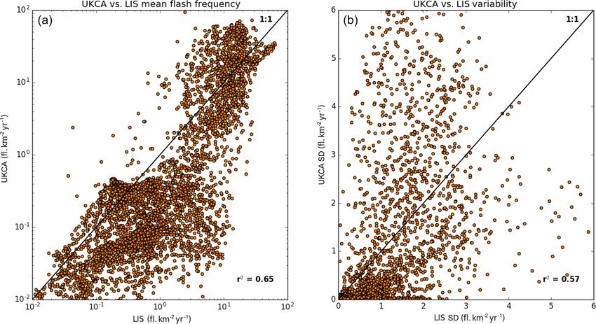
A. T. Archibald et al.: StratTrop vn 1.0                                                                                    1229

ing in vegetated regions, for most species the most important      not present an evaluation because there have been no changes
is uptake through the stomata. Through these tiny pores in         since the last published version. For an in-depth performance
the leaf surface plants take up carbon dioxide from the at-        evaluation in UKCA we refer to Sect. 3.4 in O’Connor et
mosphere and exchange water vapour and oxygen with it.             al. (2014).
This exchange also includes all other species that make up            Following a scheme originally developed by Walton et
the ambient air, including pollutants such as ozone. For this,     al. (1988) wet deposition is parameterised as a first-order
the specific type of vegetation is crucial. Ozone deposition       loss process which is calculated as a function of the three-
fluxes, for instance, vary widely between forests and grass-       dimensional convective and stratiform precipitation. The cli-
lands.                                                             mate model provides the required precipitation activity to
   The calculation of the surface resistance term and land sur-    UKCA. The wet scavenging rate r is calculated at every grid
face type information provided by the dynamic vegetation           box and time step according to
model JULES (Best et al., 2011; Clark et al., 2011) is used
in UKCA. JULES forms part of UKESM1 and is thus cou-               r = Sj × pj (l),                                           (3)
pled with UKCA. Within JULES, various land surface type
configurations may be selected. In the most simple config-         where Sj is the wet scavenging coefficient for precipita-
uration, which was also used in the UKESM1 predecessor             tion type j (cm−1 ) and pj (l) is the precipitation rate for
model HadGEM2-ES, any land-based grid box at the surface           type j (convective or stratiform), provided at model level l
can be subdivided into variable-sized fractions assigned to        (cm h−1 ).
any of nine different surface types: broadleaf trees, needle-         Scavenging coefficients for nitric acid (HNO3 ) of 2.4 and
leaf trees, C3 grasses, C4 grasses, shrubs, bare soil, rivers      4.7 cm−1 for stratiform and convective precipitation, respec-
and lakes, urban environments, and ice. Non-land grid boxes        tively, are applied (see Penner et al., 1991). These parameters
are treated separately.                                            are scaled down for individual species using the fraction of
   Since then, the number of land surface types in JULES           each species in the aqueous phase, faq , calculated by
has increased substantially (see Harper et al., 2018). Apart
                                                                             L × Heff × R × T
from the original 9-tile version (five vegetation and four non-    faq =                        ,                             (4)
vegetation types), 13-, 17- and also 27-tile configurations are            1 + L × Heff × R × T
now included. The upgrade to the 13-tile configuration in-         where L represents the liquid water content, R is the univer-
creases the number of vegetation types by introducing three        sal gas constant, T denotes ambient temperature and Heff is
broadleaf plant functional types (PFTs), two needleleaf PFTS       the effective Henry’s law constant for each species. Heff in-
and two shrub PFTS; the number of grass-related PFTs as            cludes the effects of solubility, dissociation and complex for-
well as the number of non-vegetation types remains the same        mation. Tables S6, S7 and S8 (in the Supplement) summarise
in this configuration. The 17-tile configuration further ex-       the parameters used in the UKCA wet deposition scheme
tends the number of PFTs by introducing four cropland types,       for each soluble species included in the StratTrop chemical
two C3 -grass-related and two C4 -grass-related PFTs; again,       mechanism.
the number of non-vegetation types remains the same. Fi-              Furthermore, in the scheme precipitation only occurs over
nally, the 27-tile land surface configuration, corresponding to    a fraction of the grid box. This fraction is assumed to be
the UKESM1 release configurations and the configurations           1.0 and 0.3 for stratiform and convective precipitation, re-
used for this paper, introduces a substantial number of addi-      spectively. These fractions are applied in the calculation of
tional land ice tiles. Each of these land surface and PFT tiles    the grid-box mean wet scavenging rate for both precipitation
offers a specific resistance to dry deposition of atmospheric      types after which point the two rates are added together.
gas-phase species.
   For dry deposition of aerosols a slightly different treatment   2.6   Emissions
is taken to that described above, and we direct the reader to
Mulcahy et al. (2020) and references therein for more details.     This section describes the implementation of tropospheric
                                                                   ozone precursor emissions used in the UKCA StratTrop
2.5   Wet deposition                                               scheme in detail. The scheme includes the emissions of nine
                                                                   chemical species: nitric oxide (NO), carbon monoxide (CO),
The wet deposition scheme employed in UKCA for the re-             formaldehyde (HCHO), ethane (C2 H6 ), propane (C3 H8 ), ac-
moval of tropospheric gas-phase species through convective         etaldehyde (MeCHO), acetone (Me2 CO), isoprene (C5 H8 )
and stratiform precipitation is the same as that described         and methanol (MeOH). Emissions to UKCA can be broadly
in O’Connor et al. (2014). The original scheme was im-             classified into two categories: offline, where pre-computed
plemented from the TOMCAT chemistry transport model                fluxes are read from input files, and online, where fluxes
(CTM) where it previously had been validated by Gian-              are computed in real time during the simulation by mak-
nakopoulos (1998) and Giannakopoulos et al. (1999). In this        ing use of online meteorological variables from the MetUM.
paper we provide a brief description of the scheme but will        The implementation of offline emissions will be described in

www.geosci-model-dev.net/13/1223/2020/                                                Geosci. Model Dev., 13, 1223–1266, 2020
1230                                                                                  A. T. Archibald et al.: StratTrop vn 1.0

Sect. 2.6.1. Examples of online emissions currently in UKCA        2005) inventory for the year 1990, which contains one an-
StratTrop are biogenic volatile organic compound (BVOC)            nual cycle with 12 monthly fluxes. These fluxes are applied
emissions (Sect. 2.6.2) and lightning NOx (Sect. 2.6.3). All       perpetually to all years of the time series. Biogenic emissions
emissions, including offline emissions, have interannual vari-     of acetaldehyde (MeCHO) make use of combined emis-
ability over the time period of the model simulations.             sions of MeCHO and other aldehydes from the MACCity-
   When UKCA StratTrop is coupled to the UKCA aerosol              MEGAN emissions inventory (Sindelarova et al., 2014); bio-
scheme, GLOMAP-mode (Mann et al., 2010) as here, there             genic emissions of CO, HCHO, MeOH and propane (includ-
are additional trace-gas aerosol precursor emissions for           ing C3 H6 ) are also taken from this inventory. For biogenic
dimethyl sulfide (DMS), sulfur dioxide (SO2 ) and monoter-         acetone emissions, emissions of acetone and other ketones
penes (C10 H16 ). These emissions will be discussed in the         from the MACCity-MEGAN emissions inventory (Sinde-
context of the UKESM1 aerosol performance in Mulcahy et            larova et al., 2014) are combined. Based on the years 2001–
al. (2020); the focus here will solely be on the tropospheric      2010, a monthly mean climatology is derived and applied to
ozone precursor emissions. Table S10 and Figs. S7–S8 sum-          all years (see Sect. 3 for the implementation of the emission
marise the mean global annual emissions totals for the time        in the model). Finally, soil emissions of NOx are distributed
period considered here (2005–2014) and their global and sea-       according to Yienger and Levy (1995) and scaled to give a
sonal distributions.                                               global annual total of 12.0 Tg NO yr−1 , again perpetually ap-
                                                                   plied to all years.
2.6.1   Offline anthropogenic and natural emissions
                                                                   2.6.2   Biogenic VOC emissions
Offline tropospheric ozone precursor emissions are either in-
jected into the model’s lowest layer or, in the case of aircraft   In the standard configuration of UKCA StratTrop in
emissions and some biomass burning emissions, injected into        UKESM1, emissions of organic compounds from the natural
a number of model levels. The emissions are added to the           environment (BVOC) are added to UKCA interactively (Sel-
appropriate UKCA tracers (see Table 1) and mixed simul-            lar et al., 2019). Specifically, emissions of isoprene (C5 H8 )
taneously by the boundary layer mixing scheme (Sect. 2.1).         and (mono)terpenes are online, the latter represented by a
While boreal and temperate forest and deforestation emis-          lumped compound in UKCA with the formula C10 H16 and
sions (van Marle et al., 2017) of black carbon (BC) and or-        a corresponding molecular weight of 136 g mol−1 , and cal-
ganic carbon (OC) are considered “high level” (Mulcahy et          culated by the interactive biogenic VOC (iBVOC) emission
al., 2020) and are spread uniformly up to level 20 (∼ 3 km in      model (Pacifico et al., 2011). Emission fluxes are passed to
L85), all gas-phase biomass burning emissions are added to         UKCA at every model time step.
the surface layer.                                                    In iBVOC the emissions of isoprene are coupled to the
   For anthropogenic emissions, we make use of historical          gross primary productivity of the terrestrial vegetation (Ar-
(1750–2014) annual emissions of reactive gases from the            neth et al., 2007; Pacifico et al., 2011). The biogenic emis-
Community Emissions Data System (CEDS; Hoesly et al.,              sion of all other organic compounds included in the iBVOC
2018) that were prepared for use in CMIP6. The CEDS                model, i.e. (mono)terpenes, methanol and acetone, follows
emissions are generally greater than those of other emis-          the original model described in Guenther et al. (1995). Note
sion datasets (e.g. Lamarque et al., 2010) for the years that      that the current configuration of UKCA used in UKESM1
are used in the simulations evaluated here (i.e. 2005–2014).       does not make use of the interactive emissions of methanol
Biomass burning emissions are taken from van Marle et              or acetone; these are offline as discussed in Sect. 2.6.1. To
al. (2017). They combined satellite observations from 1997         the best of our knowledge, in the case of the non-isoprene
with various proxies and output from six fire models partic-       biogenic VOCs there is no equivalent process-based formu-
ipating in the Fire Model Intercomparison Project (FireMIP;        lation for an interactive BVOC emission model applicable to
Rabin et al., 2017) to provide a complete dataset of biomass       Earth system models (ESMs).
burning emissions from 1750 to 2014 for use in CMIP6. As              For present-day conditions total global annual emissions
was the case for anthropogenic emissions, emissions from           of isoprene amount to 495.9 (± 13.6) Tg C yr−1 . This num-
the years 2005–2014 are used here. For both anthropogenic          ber represents the 10-year average annual total emission
and biomass burning, the emissions were re-gridded from            strength and the uncertainty quantified by the standard devi-
their native resolution to N96L85 while conserving global          ation over the 10-year period between 2005 and 2014 taken
annual totals and seasonal cycles. Emissions of all C2 and C3      from a historic run with UKESM1 (Sellar et al., 2019). This
VOCs are included as ethane and propane, respectively.             is in good agreement with estimates reported for other emis-
   For natural emissions which are not simulated, offline          sion models (e.g. Arneth et al., 2008; Guenther et al., 2012;
emissions are prescribed through the provision of pre-             Messina et al., 2016; Müller et al., 2008; Sindelarova et al.,
computed fluxes. For example, oceanic emissions of CO,             2014; Stavrakou et al., 2009; Young et al., 2009). For the
ethane (including ethene – C2 H4 ) and propane (including          global annual total (mono)terpene emissions, iBVOC calcu-
propene – C3 H6 ) are taken from the POET (Granier et al.,         lates 115.1 (± 1.6) Tg C yr−1 over the same period of model

Geosci. Model Dev., 13, 1223–1266, 2020                                             www.geosci-model-dev.net/13/1223/2020/
A. T. Archibald et al.: StratTrop vn 1.0                                                                                        1231

Figure 1. Tropical distribution of the LIS-observed (Lightning Imaging Sensor) climatological annual mean lightning flash density over
the period 1999–2013 (a) in comparison with the modelled annual mean climatology from the period 2005–2014 (b). The corresponding
standard deviation of the observed and modelled climatologies are shown in panels (c) and (d), respectively.

simulation. This model estimate is in reasonably good agree-         (3.0 ×10⁹ J flash−1 ) being approximately 3 times greater
ment with the literature (e.g. Folberth et al., 2006; Lathière       than that for cloud-to-cloud (0.9 ×10⁹ J flash−1 ) flashes
et al., 2006; Arneth et al., 2007, 2011; Acosta Navarro et al.,      (Schumann and Huntrieser, 2007).
2014; Sindelarova et al., 2014; Bauwens et al., 2016; Messina           This implementation is identical to that implemented
et al., 2016).                                                       in HadGEM2-ES (Collins et al., 2011) by O’Connor et
   In the configuration of UKCA StratTrop used in                    al. (2014) except that NOx emissions are now distributed
UKESM1, isoprene is included in the gas-phase chemistry              linearly in log(pressure) rather than linearly in pressure.
but does not contribute to the formation of secondary organic        Whereas global annual lightning emissions in HadGEM2-
aerosol (SOA). Emissions of (mono)terpenes are oxidised us-          ES were inadvertently too low (O’Connor et al., 2014;
ing a fixed yield approach (e.g. Kelly et al., 2018) to form         Young et al., 2013), here the emissions have been scaled
SOA in the GLOMAP-mode aerosol scheme – see Table S1                 to give an average global annual emission rate of 5.93 and
and Mulcahy et al. (2020) for a detailed description and eval-       5.98 Tg N yr−1 over the period 2005 to 2014 in the free-
uation.                                                              running and nudged simulations, respectively. When com-
                                                                     pared with anthropogenic, biomass burning and natural emis-
2.6.3   Emissions of NOx from lightning                              sions, lightning contributes approximately 10 % to the global
                                                                     annual NOx emission rate, consistent with estimates from
The lightning NOx emissions scheme in UKCA StratTrop is              Schumann and Huntrieser (2007).
based on the cloud-top parameterisation proposed by Price               Figure 1 shows tropical distributions of decadal mean an-
and Rind (1992). Based on satellite data and storm measure-          nual flash density as observed by the Lightning Imaging Sen-
ments, the lightning flash density is parameterised as               sor (LIS) onboard the Tropical Rainfall Measuring Mission
Fl = 3.44 × 10⁻⁵ H 4.9 ,                                     (5)     (TRMM) satellite (Theon, 1994) in comparison with the free-
                                                                     running simulation being evaluated here (see Sect. 3 for de-
Fo = 6.2 × 10⁻⁴ H 1.3 ,                                      (6)     tails). It demonstrates that UKCA is capable of capturing the
where F is the flash density   (flash min−1 ),
                                            H is the cloud-          broad features of the observed climatology, with peak den-
top height (km), and the “l” and “o” subscripts are used             sities over South America, Africa and East Asia; the spatial
to represent the land and ocean, respectively, and to dis-           coefficient of determination (R 2 ) between the modelled and
tinguish between the updraft velocities experienced over             observed climatology is 0.65 and 0.69 in the free-running and
the two surfaces. The scheme also differentiates between             nudged (not shown) simulations, respectively. However, the
cloud-to-cloud and cloud-to-ground flashes based on the              model tends to be biased low in regions of low flash density
grid cell latitude (Price and Rind, 1993) and is resolution-         (e.g. over the oceans and towards the extratropics) compared
independent by the implementation of a spatial calibra-              to the observations (Fig. 2), consistent with the assessment of
tion factor (Price and Rind, 1994). A minimum cloud                  Finney et al. (2014). In considering the variability, the spatial
depth of 5 km is required for NOx emissions to be ac-                R 2 between the modelled and observed standard deviation
tivated and is diagnosed on a time-step basis from the               is 0.57 and 0.59 in the free-running and nudged simulations,
physical model’s convection scheme. For NOx production,              respectively. The variability from UKCA is comparable in
the parameterisation assumes that the production efficiency          magnitude to that observed over Africa, albeit displaced ge-
per unit of energy discharged is 25 ×1016 molec NO J−1 ,             ographically. Over the Maritime Continent and South Amer-
with the energy discharged from cloud-to-ground flashes

www.geosci-model-dev.net/13/1223/2020/                                                  Geosci. Model Dev., 13, 1223–1266, 2020
1232                                                                                          A. T. Archibald et al.: StratTrop vn 1.0

Figure 2. Scatter plot of the modelled versus the LIS-observed multi-annual mean lightning flash density (a) and the standard deviation (b).

ica, for example, UKCA overestimates the variability relative           Table 2. List of halocarbons (not explicitly treated in the model)
to the LIS observations.                                                contributing to the lower boundary conditions of CFC-11, CFC-
   Whilst the skill of the cloud-top parameterisation is good           12 and CH3 Br. Note that H-1211 contributes to both CFC-11 and
relative to other parameterisations (Finney et al., 2014), and          CH3 Br as it contains both Cl and Br. Contributions are included by
the performance here in the free-running and nudged model               moles of Cl or Br.
simulations is consistent with that assessment, raising the di-
                                                                                        CFC-11         CFC-12        CH3 Br
agnosed cloud-top height over land to the power of 4.9 makes
the cloud-top parameterisation susceptible to model biases in                           CCl4           CFC-113       H-1211
cloud-top height, as noted by Allen and Pickering (2002) and                            CH3 CCl3       CFC-114       H-1202
Tost et al. (2007). Lightning is potentially a key chemistry–                           HCFC-141b      CFC-115       H-1301
climate interaction in Earth system models, but the sensitivity                         HCFC-142b      HCFC-22       H-2402
                                                                                        H-1211
to how it is represented (i.e. using cloud-top height (Baner-
                                                                                        CH3 Cl
jee et al., 2014) or ice-flux-based parameterisations; Finney
et al., 2018) warrants further investigation. Indeed, Hakim et
al. (2019) recently identified uncertainty in modelled light-
ning NOx in the Indian subcontinent as being an important               on 1 July for each year specified and are linearly interpolated
source of uncertainty in model simulations of tropospheric              in time to give daily values if data for more than one time
ozone in that region.                                                   point are defined. CFC-11, CFC-12 and CH3 Br also contain
                                                                        contributions from other Cl- and Br-containing source gases
2.6.4   Lower boundary conditions                                       which are not explicitly treated in the model to ensure that
                                                                        there is the correct stratospheric chlorine and bromine load-
Lower boundary conditions are provided at the surface for               ing, with these contributing species given in Table 2. These
the chemical species CH4 , N2 O, CFC-11 (CFCl3 ), CFC-12                values are converted into a two-dimensional “effective emis-
(CF2 Cl2 ), CH3 Br, H2 and COS. Values for H2 and COS are               sion” field at each time step that is used to fix the surface
fixed at 500 ppb and 482.8 ppt, respectively (invariant with            concentrations of these species.
time). Values for the remaining species are specified using
time series data provided for the 5th Coupled Model Inter-
comparison Project (CMIP5) for the greenhouse gas concen-
trations (RCP Database, 2020). The values provided are valid

Geosci. Model Dev., 13, 1223–1266, 2020                                                     www.geosci-model-dev.net/13/1223/2020/
A. T. Archibald et al.: StratTrop vn 1.0 1233
2.7 Coupling with other Earth system components heterogeneous uptake. In UKCA StratTrop, γ N2 O5 is set at
this higher value, 0.1, throughout the atmosphere. In part this
Secondary aerosol formation of sulfate and organic carbon compensates for the fact that there is an important missing
in UKESM1 (Sellar et al., 2019) is determined by oxidants aerosol surface in UKESM1 in the troposphere in the form
(OH, O3 , H2 O2 , NO3 ) modelled interactively by the UKCA of nitrate aerosol. The lack of nitrate aerosol is an issue
StratTrop chemistry scheme. For further details on the ox- for UKESM1 simulations of particulate matter, particularly
idation of sulfate and SOA precursors, chemistry–aerosol in regions with high levels of ammonia emissions. An im-
coupling, and the scientific performance of the aerosol proved understanding of γ N2 O5 is needed to understand both
scheme (GLOMAP-mode; Mann et al., 2010) in UKCA and the current composition and the combined impact of chang-
UKESM1, the reader is referred to Mulcahy et al. (2020). ing gas- and aerosol-phase composition. Whilst more so-
In the HadGEM2-ES model (Collins et al., 2011) used phisticated treatments of γ N2 O5 are available (e.g. Bertram
for CMIP5, radiative feedbacks between UKCA-modelled and Thornton, 2009) and have been included in versions of
methane and tropospheric ozone concentrations were active UKCA, further work is required to improve this aspect of the
(OC14); stratospheric ozone was prescribed and combined mechanism for UKCA in UKESM1.
with the modelled interactive tropospheric concentrations.
In UKESM1 (Sellar et al., 2019), however, the coupling 2.7.2 Chemical production of H2 O
between the UKCA-modelled radiatively active trace gases
and the radiation scheme has been extended to include N2 O There are many chemical reactions which consume or pro-
and stratospheric ozone (in addition to methane and tropo- duce water vapour in the troposphere and stratosphere. For
spheric ozone). Although chlorofluorocarbons (CFCs) and example, reactions between the hydroxyl radical (OH) and
hydrochlorofluorocarbons (HCFCs) are modelled in UKCA VOCs usually result in the production of a water molecule.
StratTrop, the radiation scheme cannot handle the speci-
OH + VOC → H2 O + organic radical (7)
ation. Therefore, separate lumped species (CFC12-eq and
HFC134a-eq) are prescribed in the radiation scheme (see In the troposphere the chemical source of water vapour is
Sect. 2.6.4 on how the lumping and mapping is done). negligible compared with that from the oceans and evapo-
transpiration from the Earth’s land surface, but given the low
2.7.1 Heterogeneous chemistry couplings temperatures around the tropopause, chemically produced
water is very important in the lower stratosphere. Further-
In UKCA StratTrop as implemented in UKESM1, five dif- more, the main source of chemical water in the middle to up-
ferent heterogeneous reactions are included (see Table S4). per stratosphere comes from the oxidation of CH4 . Complete
These reactions occur on the modelled soluble aerosol sur- oxidation of CH4 to CO2 can result in the net production of
face area, which in the troposphere is calculated interac- two water molecules.
tively using GLOMAP-mode by summing over all soluble In previous versions of UKCA, such as that used in
aerosol modes. In the stratosphere (defined here as being HadGEM2-ES, the oxidation of CH4 to produce chemical
12 km above the surface) the aerosol surface area comes from water was neglected. Instead, stratospheric water vapour was
the stratospheric sulfate surface area density input climatol- simulated using the following simple relationship:
ogy, discussed in Sellar et al. (2020). The combining of the
stratospheric aerosol surface area density from the climatol- 2 × [CH4 ] + [H2 O] = 3.75(ppm), (8)
ogy and the interactive components of GLOMAP-mode is
calculated at each UKCA time step, and only the soluble where UKCA was used to calculate [CH4 ]. In UKCA Strat-
aerosol modes simulated by GLOMAP are included in the Trop as implemented in UKESM1 we now include inter-
calculation. active H2 O production from all chemical reactions in the
Heterogeneous reactions are extremely important for sim- mechanism. In this way UKCA now passes the water vapour
ulating composition change in the stratosphere (Keeble et field after the chemistry step back to the main climate model
al., 2014), and there is increasing attention to the simula- where it is used in other routines. The annual mean zonal-
tion of these processes in the troposphere (e.g. Jacob et al., mean chemical production of H2 O as simulated by UKESM1
2000; Lowe et al., 2015). One of the most important tropo- is shown in Fig. 3. There are two clear regions which domi-
spheric heterogeneous reactions is that of N2 O5 on aerosol nate where H2 O chemical production takes place: in the trop-
surfaces (Jacob et al., 2000). This reaction is complicated ical lower troposphere and the tropical upper stratosphere. In
because of the dependence of the uptake parameter (γ ) on both regions the primary source of chemical water is the oxi-
the composition of the aerosol as well as on temperature dation of CH4 . Figure 3 compares the absolute production of
and relative humidity (Bertram and Thornton, 2009). Mac- chemical water (panel a) and the production of chemical wa-
intyre and Evans (2010) suggest that models that use high ter as expressed in mixing ratio units (panel b). In this sense,
values of γ N2 O5 (∼ 0.1) overestimate the impact of chang- panel (b) shows that the relative production of chemical wa-
ing aerosol loadings on tropospheric composition through ter is greatest in the upper stratosphere. The contribution of
www.geosci-model-dev.net/13/1223/2020/ Geosci. Model Dev., 13, 1223–1266, 20201234 A. T. Archibald et al.: StratTrop vn 1.0
Figure 3. Multi-annual mean zonal-mean production of H2 O from the UKCA StratTrop mechanism in UKESM1. Panel (a) shows the
production in moles per second and panel (b) in parts per billion per day, highlighting the larger relative source of water from chemical
processes in the upper atmosphere.
this source of stratospheric H2 O to the present-day forcing of tivity to different (a) rate coefficients (updating the JPL and
climate relative to the pre-industrial period will be assessed IUPAC recommendations), (b) reactions (by looking at the
in O’Connor et al. (2019). sensitivity to specific reactions associated with isoprene oxi-
dation (Archibald et al., 2011) and the reaction between HO2
2.7.3 Future couplings and NO; Butkovskaya et al., 2005, 2007, 2009), (c) treat-
ment of photolysis, (d) emissions and (e) deposition param-
Although UKESM1 (Sellar et al., 2019) represents a signifi- eters. These one-at-a-time simulations are outlined in Ta-
cant enhancement in the representation of atmospheric chem- ble S9 in the Supplement. It should be noted that these sim-
istry and Earth system interactions, a number of key interac- ulations provide an ensemble of opportunity; they were not
tions are not included. For example, the coupling of aerosols designed to probe model sensitivity in a targeted way. How-
with Fast-JX is omitted despite the impact of aerosols on the ever, they result in some useful information which helped the
tropospheric photochemical production of ozone (e.g. Xing development of the StratTrop mechanism. These simulations
et al., 2017; Wang et al., 2019). This development is currently made use of an older version of the MetUM and an ear-
underway and will be included in future versions of UKCA lier atmosphere-only version of UKCA, which is now dep-
and UKESM. Ozone damage to natural and managed ecosys- recated. That version of UKCA ran at a lower resolution than
tems (e.g. Ashmore, 2005) has an important impact on the the version discussed in this paper and used in UKESM1
strength of carbon uptake by vegetation (Sitch et al., 2007; (about half the resolution). The results from these simula-
Oliver et al., 2018) and has yet to be implemented. In addi- tions are shown in Fig. 4 where they are compared against
tion, although the terrestrial carbon cycle considers nitrogen results from model intercomparison studies (further analy-
availability and limitation, nitrogen deposition rates are pre- sis of the model sensitivity tests is presented in Figs. S1–
scribed in UKESM1; future work will include implementing S6 in the Supplement). Figure 4 focuses on a subset of the
a nitrate aerosol scheme in GLOMAP-mode and coupling the full range of experiments performed but contextualises these
deposition of both oxidised and reduced nitrogen from the at- by comparing to results from the ACCENT simulations dis-
mosphere to the terrestrial biosphere. cussed in Stevenson et al. (2006) (black dots) and the AC-
CMIP simulations discussed in Young et al. (2013) (orange
2.8 Historic development of the chemistry scheme dots). In addition to the early sensitivity tests (the blue dots
in Fig. 4), we also show the results from the simulations pre-
During the development of the StratTrop chemistry scheme,
sented here, labelled UKESM1 (red triangle in Fig. 4). The
several simulations were run to test the scheme and its sensi-
Geosci. Model Dev., 13, 1223–1266, 2020 www.geosci-model-dev.net/13/1223/2020/A. T. Archibald et al.: StratTrop vn 1.0 1235
cal loss flux (grey arrow), indicating increased photochem-
ical activity. The attribution of which rate coefficients were
dominant in this behaviour is outside the scope of this work.
Similarly, we note that the metrics analysed are sensitive to
lightning NOx (Banerjee et al., 2014); decreasing the light-
ning NOx emissions by 50 % (to ∼ 3 Tg yr−1 ) results in an in-
creased methane lifetime of ∼ 1 year (purple arrow). Figure 4
also highlights a non-linear response in the simulations to
changes in isoprene emissions; scaling them by a factor of 2
(100 % increase and 50 % decrease; green arrows) leads to a
highly non-linear response in the metrics analysed. Finally,
we note that the change which had the biggest impact on
the metrics was switching to the FAST-JX photolysis scheme
(Telford et al., 2013) from precalculated photolysis rates and
a lookup table (pink arrow). The main reason for this is that
Figure 4. Comparison of early tests of the StratTrop scheme run- the precalculated photolysis rates had underestimated rates
ning in an older version of UKCA (blue dots) with the scheme for the photolysis of O3 to O(1 D). This behaviour has been
applied in UKESM1 (red triangle; free-running simulation), other documented previously (Voulgarakis et al., 2009; Telford et
CCMs which took part in the ACCMIP intercomparison (orange al., 2013).
dots) and CTMs which took part in the ACCENT intercomparison
In addition to the tests described above we found during
(black dots). The letters in the legend (i.e. B–A) refer to the experi-
ments outlined in Table S9.
the testing of the StratTrop scheme that inclusion of the ter-
molecular reaction
HO2 + NO + M → HONO2 + M, (9)
figure focuses on the relationship between methane lifetime
which has been shown to exhibit both pressure and water
and ozone chemical loss, important metrics for represent-
vapour dependence (Butkovskaya et al., 2005, 2007, 2009),
ing key sources and sinks of tropospheric OH (Wild, 2007).
led to large changes in the metrics analysed in Fig. 4 (see
Both metrics are calculated by masking out the stratosphere.
Sect. S1.2 of the Supplement for further details). Previous
The methane lifetime is calculated by dividing the burden of
modelling work highlighted that this could have an impor-
methane in the model by the reaction flux between methane
tant impact on the simulation of ozone (Cariolle et al., 2008).
and OH in the troposphere, so it represents the lifetime with
However, owing to uncertainty in its recommendation be-
respect to OH in the troposphere. The ozone loss is calculated
tween the recent evaluations by JPL and IUPAC we have
by summing the reaction fluxes which are key for O3 loss in
omitted it from the StratTrop scheme used in UKESM1.
the troposphere (reactions of O3 with HOx species and the re-
action between O(1 D) and H2 O). The experiments outlined
in Table S9 and shown in Fig. 4 emphasise that the range in 3 Model simulations to evaluate UKCA StratTrop in
O3 loss and CH4 lifetime spanned by changing aspects of the UKESM1
UKCA model span a range as wide as that covered by the
ACCMIP models (Young et al., 2013). In other words, the In this section, we discuss a series of simulations that
ensemble of opportunity from the early tests of the UKCA have been performed to evaluate the performance of the
StratTrop scheme span as wide a range in the metrics pre- UKCA StratTrop scheme in UKESM1. These simulations
sented as the structurally different ACCMIP and ACCENT link closely to the UKESM1 historical and AMIP simula-
models. Interestingly, the UKESM1 simulations discussed in tions by using similar inputs, e.g. emissions, and crucially
this paper in detail lie close to the ACCENT ensemble (black the version of UKCA StratTrop is identical to that used in
dots), yet the early test simulations using the same chemi- UKESM1 (Sellar et al., 2019).
cal mechanism but an earlier version of the MetUM model Simulations analysed in this paper have been carried out
do not (the blue cluster of dots). This highlights that struc- with an atmosphere-only configuration of UKESM1 (Sellar
tural changes in the underlying meteorological model can et al., 2019). The sea surface temperatures and sea ice cover
substantially influence key metrics of atmospheric compo- used to drive the model are those specified for the historical
sition through changes in the distribution of clouds, water period by the Sixth Coupled Model Intercomparison Project
vapour and other key variables. (CMIP6 project; Durack et al., 2016). Land cover fraction,
These sensitivity studies highlight some important points. vegetation canopy height and leaf area index (LAI) have been
Simulations using kinetic data recommendations from IU- provided as multi-annual monthly mean climatologies de-
PAC and JPL updated from 2005 to 2011 led to a decrease rived from a historical simulation of UKESM1, which in-
in model methane lifetime and an increase in ozone chemi- cludes the dynamic vegetation model TRIFFID (Cox, 2001).
www.geosci-model-dev.net/13/1223/2020/ Geosci. Model Dev., 13, 1223–1266, 2020You can also read