Detecting Emotions in English and Arabic Tweets - MDPI
←
→
Page content transcription
If your browser does not render page correctly, please read the page content below
information
Article
Detecting Emotions in English and Arabic Tweets
Tariq Ahmad 1, * , Allan Ramsay 1               and Hanady Ahmed 2
 1   School of Computer Science, The University of Manchester, Oxford Road, Manchester M13 9PL, UK;
     allan.ramsay@manchester.ac.uk
 2   CAS, Arabic Department, Qatar University, Al Hala St, P.O. Box 2713 Doha, Qatar; hanadyma@qu.edu.qa
 *   Correspondence: tariq.ahmad@postgrad.manchester.ac.uk; Tel.: +44-161-275-2611

 Received: 21 January 2019; Accepted: 28 February 2019; Published: 6 March 2019

 Abstract: Assigning sentiment labels to documents is, at first sight, a standard multi-label classification
 task. Many approaches have been used for this task, but the current state-of-the-art solutions use
 deep neural networks (DNNs). As such, it seems likely that standard machine learning algorithms,
 such as these, will provide an effective approach. We describe an alternative approach, involving the
 use of probabilities to construct a weighted lexicon of sentiment terms, then modifying the lexicon
 and calculating optimal thresholds for each class. We show that this approach outperforms the use of
 DNNs and other standard algorithms. We believe that DNNs are not a universal panacea and that
 paying attention to the nature of the data that you are trying to learn from can be more important than
 trying out ever more powerful general purpose machine learning algorithms.

 Keywords: sentiment mining; shallow learning; multi-emotion classification

1. Introduction
     There are many ways to detect emotion. Quintana et al. [1] showed how to recognise emotion
using the variability of heart rate. Nakasone et al. [2] used electromyography and skin conductance to
determine emotion, and Busso et al. [3] recognised emotions using facial expressions and speech. This
paper focuses on detecting emotions from documents.
     According to recent research by Young et al. [4], deep learning methods are currently the
state-of-the-art results in many domains. This trend was confirmed by the number of entries in
the recent SemEval-2018 competition [5], where the winning entries in the English and Spanish [6,7]
multi-classification competition all made use of neural networks. Indeed, many of the top-performing
entries made use of a special kind of neural network known as “long short-term memory”, either
in conjunction with attention mechanisms [8,9], word embeddings [10,11] or convolutional neural
networks [12,13].
     The key features when trying to assign sentiment labels to documents are the words that they
contain. Most approaches to this task involve the explicit or implicit construction of a sentiment lexicon.
We explore two ways of constructing such a lexicon, either by explicitly counting the occurrences of
words in documents that have been assigned a (possibly empty) set of labels drawn from a standard
set of sentiment names or by building a deep neural network (DNN) with the set of words in the
training set as input features and the sentiment names as output features. In the latter case, the lexicon
is implicit in the weights that link the input layer, via the hidden layers, to the output layer. Such an
implicit lexicon is often referred to as a word embedding; in essence, however, it is just a lexicon where
each word is connected to a set of labels through a collection of arithmetical calculations.
     Given that the task we are undertaking involves assigning a set of labels, we have to be careful
about how we use DNNs. There are two obvious ways to proceed. (i) Given a set of features, it would
be possible to train a set of classifiers, one per feature. Each classifier will return YES/NO for the

Information 2019, 10, 98; doi:10.3390/info10030098                        www.mdpi.com/journal/information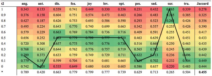
Information 2019, 10, 98                                                                              2 of 20

feature on which it was trained. Taken together the set of classifiers can be seen as a single multi-label
classifier. We refer to classifiers trained in this way as multi-DNNs. (ii) Train a single classifier with a
node in the output layer for each feature and then accept every label for which the output-layer node
had an excitation level above some threshold. We refer to this kind of classifier as single-DNN.
     Emotion classification tasks have traditionally been tackled by obtaining a large corpus, constructing
feature sets, pre-processing in sophisticated ways and then making use of any number of black box
training algorithms [14,15]. Indeed, this approach is still prevalent currently [6,7,16]. We demonstrate
that with a small-sized corpus and without using any black box algorithms, our results are comparable
with systems that have been trained on millions (and sometimes billions) of tweets.
     We show that the approach through explicitly constructing a lexicon substantially outperforms
both of the DNN algorithms outlined above, and we speculate about why this should be so.

2. Materials and Methods

2.1. Data Collection
      We used the data provided for the SemEval-2018 Task 1: Affect in Tweets task for English and
Arabic. The organisers provided training, development and test datasets of tweets in Arabic and English.
The tweets in the training and development datasets were each labelled with a (possibly empty) set of
emotions. To create the English datasets, firstly, 50–100 terms were selected for each emotion. These
were terms that were associated with the emotion, but at different intensity levels (e.g., for “angry” the
terms “mad”, “frustrated”, “annoyed”, “peeved”, “irritated”, “miffed”, “fury” and similar terms were
used). These were either obtained from Roget’s Thesaurus or were nearest neighbours of the emotion
words in a word-embedding space. Twitter was polled for the period June–July 2017 for tweets that
included these query terms, and tweets were randomly selected for annotation. Finally, 100 tweets
that had an emotion-word hashtag, emoticon or an emoji query term at the end were selected for
each emotion, and the trailing query term was removed. Consequently, the final dataset also included
tweets that contained no clear terms that indicated the emotion. The Arabic dataset was constructed
in a similar fashion, but the English query terms were translated into Arabic using Google Translate,
and EmoLex [17] was used to find words associated with the emotions. The authors describe how
17 million tweets were collected by polling Twitter for tweets that included emotion-related words such
as “angry”, “annoyed”, “panic”, “happy”, “elated”, “surprised”, etc. The full list of query terms, for
both languages, is available in their paper [18].
      It is worth noting here that the Arabic tweets typically contained more words than the English
ones. Arabic tweets had an average of 27 words, whereas for English tweets, it was 16. We believe
that this reflects the fact that Arabic is typically written in a very condensed form, in which the marks
corresponding to short vowels and other phonetically-relevant items (diacritics) are omitted. This is
similar to the use of “textese” in English, wherein a text like “This message is heavily abbreviated” might
be written as “This msg is hvly abbrvted”. The omission of diacritics from written Arabic introduces more
ambiguity than is the case for English written as textese; this makes Arabic tweets harder to analyse
than English tweets. At the same time, it also means that it is possible for there to be significantly more
words in an Arabic tweet than an English tweet. In a sense, this makes the task easier, since the more
words there are, the more information there is about what the tweet says. As we will show, the results
we obtained for the English and Arabic sets were extremely similar; hence, we believe these two effects
cancelled each other out.
      Having obtained tweets using the query terms, Mohammad et al. used a “somewhat generous”
criteria when deciding which tweets to include in the dataset. Seven people were asked to annotate
the tweets, and if at least two indicated that a certain emotion was inferred, then that emotion was
chosen as one of the labels for the tweet.
      It was surprising to see the relatively low annotator agreement levels; 0.48 for the Arabic
dataset and 0.40 for the English dataset. These fall into the “moderate agreement” [19] band in
Information 2019, 10, 98                                                                                   3 of 20

the interpretations of Fleiss’ kappa, indicating that the annotation was not a straightforward task due
to its subjective nature.
      Low annotator agreement is not uncommon. For example, Purver and Battersby [20] found very
little agreement between the annotators when they manually labelled tweets with Ekmans [21] six
emotions. Similarly, the work in [22–24] all reported low levels of inter-annotator agreement.
      There were a number of interesting observations:

•     There were more emotions than tweets in each dataset; this was to be expected since tweets can,
      and often do, contain multiple emotions.
•     There were approximately the same number of average emotions per tweet across all four datasets;
      it is not clear whether this is by design or naturally occurring.
•     The distributions of emotions across datasets from the same language were similar and, in some
      cases, (e.g., anger) were the same across all the datasets.
•     Table 1 shows the breakdown of tweets by emotion. The table also shows that anger was the
      most popular emotion. Anger is an emotion that manifests itself by hostility towards someone
      or something. According to psychologists, anger can be a “substitute” emotion, meaning that
      people can make themselves angry so that they do not have to experience an even worse emotion
      such as pain. Fan et al. [25] collected 70 million tweets from Sina Weibo (a Chinese microblogging
      website) to examine how tweets that channelled specific emotions (joy, sadness, anger and disgust)
      influenced other people across the site. They found that “the most observable pattern was in the
      spread of angry tweets”. This means that if a user sent an angry tweet, that anger emotion is likely
      to leak into the tweets of not only the followers who saw the tweet, but also their followers, and
      their followers’ followers. They concluded that anger spreads faster than any other emotions
      on Twitter, and this could help explain why anger is the most popular emotion in the SemEval
      2018 datasets. The next most popular emotion was sadness, followed closely by joy, possibly
      for similar reasons. At the opposite end of the scale are surprise and trust. This is likely because
      aside from the emotion words themselves, there are not many other words that convey these
      emotions. Furthermore, these are hardly emotions that one would see being shared amongst
      social media users.

     The final datasets (the datasets are available from https://competitions.codalab.org/competitions/
17751#learn_the_details-datasets) consisted of a training set of around 6.8K English tweets (109K words)
and 2.2K Arabic ones (62K words) and development sets of around 886 tweets (13.9K words) and
586 tweets (15.8K words), respectively.

                              Table 1. SemEval-2018 tweets by emotion (percentages).

                Dataset        ang.   ant.   dis.   fea.   joy   lov.   opt.   pes.   sad.   sur.   tru.
           Arabic training      17     4      8      6     12    12     12     10      16     1      2
             Arabic test        16     4      8      7     12    12     12      9      16     1      3
           English training     16     6     16      8     16    4      12     5       13     2      2
             English test       15     6     15      6     18    5      14     5       12     2      2

2.2. The Task
     The task (named Task “E-c” in the competition) was to classify each tweet in the test set as “neutral
or no emotion” or as one, or more, of eleven given emotions, {anger, anticipation, disgust, fear, joy, love,
optimism, pessimism, sadness, surprise and trust}, that best represented the mental state of the tweeter.

2.3. Algorithm
      Our weighted conditional probabilities (WCP) strategy was based on:

1.    Using the tweets in the annotated training dataset to create word vectors.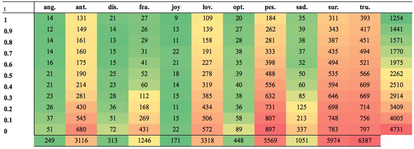
Information 2019, 10, 98                                                                              4 of 20

2.    Using the word vectors to create a lexicon of tokens and conditional probabilities.
3.    Transforming the probabilities into “scores”.
4.    Autocorrecting the lexicon by iteratively using a range of thresholds to remove unhelpful words.
5.    Using the modified lexicon to calculate the threshold that achieved the best results for each emotion.
6.    Classifying the test data using the modified lexicon and the best set of thresholds.

    The outcome of this process was a trained model that could be used to classify the unseen,
unannotated, tweets in the test dataset. Figure 1 shows an overview of the methodology architecture.
Each stage is explained in further detail in this section.

                                       Figure 1. Architecture diagram.

2.3.1. Preprocessing
      Preprocessing is an important and crucial step to obtaining good results; hence, each tweet was
preprocessed, and a set of tokens and a count of each distinct token in the tweet were obtained. Tweets
were preprocessed by lowercasing (English tweets only), removing Arabic and English punctuation,
identifying and replacing emojis with emoji identifiers, expanding hashtags and then tokenising
and stemming.
      We believed that multi-word hashtags (e.g., #better_world, #late-night) also contained useful
information. Consequently, to improve the quality of information in the tweet, hashtags were left
unaltered, but a copy of the hashtag was taken and split into its constituent words (“expanded”).
      Two tokenisers were developed for use on both languages: one was based on the Natural
Language Toolkit (NLTK) [26] and did not preserve hashtags, emoticons, punctuation and other
content, and one was “tweet-friendly” because it preserved these items.
      As the name suggests, emojis are used to convey emotions and hence were very significant for
the current task. It was tricky to identify them, since the set is not fixed, and they also caused many
technical problems due to their surrogate-pair nature. Hence, these were replaced with emoji identifiers
(e.g., _45_). Contiguous instances of emojis were also separated out. This is because the individual
emojis in a group of repeating unhappy face emojis should be recognised, and processed, as being
the same emoji as a single unhappy face emoji. Usernames were also removed because we believed
they were noise, since, by and large, they did not reappear in the test set, were not helpful and if left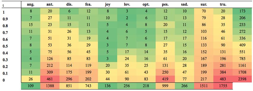
Information 2019, 10, 98 5 of 20
in would compromise the ability to detect useful information and would add, unnecessarily, to the
computational load.
Up to this point, the steps for both languages were the same.
Stemming the words that appeared in a tweet was challenging, since the vocabulary used in tweets
was very open and included numerous slang items and (deliberate and accidental) misspellings, so that
stemmers that relied on a fixed lexicon (e.g., Madamira for Arabic [8]) did not work well on tweets.
Arabic and English tweets were tagged and stemmed in different ways.
2.3.2. Arabic Tagging and Stemming
Two techniques were developed to stem Arabic tweets, a “simple” method and a more complex
method.
In the simple method, there was no explicit tagging stage. The token was simply firstly stemmed
as a noun and then again as a verb using the stemmer developed specifically for Arabic tweets by
Albogamy and Ramsay [27]. The shortest answer returned (in terms of the number of characters) was
then taken as the answer. For example, when the Arabic word àñPYK (they study, present tense,
masculine, plural) was stemmed as a noun, the result was
PYK (he studies, present tense, masculine,
singular); when it was stemmed as a verb, the result was PX (he studied, past tense, masculine,
singular). In this example, therefore, the verb form was taken as the correct stemmed form.
In the second method, Albogamy and Ramsay’s tagger [28] was firstly used to establish the tag
(noun, verb, etc.). This tag was then used to stem the word, again using the stemmer developed by
Albogamy and Ramsay [27].
2.3.3. English Tagging and Stemming
Two similar techniques were also developed to stem English tweets. In the simple method, tweets
were stemmed by, again, taking the shortest result from Morphy [29] when tokens were stemmed as
nouns, verbs, adjectives and adverbs. Consider the following example (not from Morphy): the word
“beautiful” has many different forms, such as beauty (noun), beautify (verb), beautiful (adjective) and
beautifully (adverb). In this example, the noun would be taken as the correct stemmed form.
In the second method, the NLTK parts-of-speech tagger was used to generate the tags for the
tokens. These tokens were then mapped to Morphy tokens, and Morphy was used to stem the word
with the derived tag.
These preprocessed tokens were used to create counts of the number of tweets each token
appeared in, and the reciprocal of each of these values was calculated to create an inverse document
frequency (IDF) vector.
Common words such as “a” and “i” had scores close to 0, whereas words that did not commonly
appear had higher scores and were, thus, more important.
2.3.4. From Probabilities to Scores
Manual inspection of the distinct tokens showed that taking the top 2500 tokens appeared to be a
good compromise between ignoring uncommon tokens and ensuring that the important tokens were
captured. The most important tokens were extracted by, firstly, removing singletons (tokens that only
occurred once in the dataset) and then simply taking the top 2500 tokens with the smallest IDF values
(recall, IDF is small for commonly-used words and bigger for words that are used infrequently).
Ignoring uncommon tokens was important because, realistically, it could not be expected that place
names, product names and brand names would be useful. Furthermore, since these words occurred
very infrequently, it was unlikely to be possible to learn anything from them, and as they had little
effect on the overall results, they only added extra unnecessary computational workload. Note that the
words themselves remained present in the tweets; their scores were simply adjusted in the lexicon.Information 2019, 10, 98 6 of 20
Our approach was firstly to create probabilities and then to use these probabilities as a basis for
constructing “scores”. The probabilities were not used to construct scores for the individual emotions,
but instead to construct scores relative to the other emotions. Constructing scores in this manner
allowed us to make the observation that words such as “blessed” were much more significant for
emotions such as joy, love and optimism than they were for emotions such as anger and anticipation and
also then to take appropriate actions. Words that were insignificant had small scores, whereas words
that were significant had large scores.
Lexicon
A base lexicon was created that contained every token in every tweet and a count of how often
the token occurred against each of the emotions.
Tokens like “a” and “the” appeared many times across all emotions; consequently, they were of
little importance. However, highly emotive tokens such as “rage” and “fury” appeared less frequently,
but, crucially, appeared highly in negative emotions. A count of the number of tokens in each emotion
was also obtained.
Raw Conditional Probabilities
For all tokens Ti and all emotions Ej , the conditional probability P( Ti | Ej ) that a tweet that
expresses the emotion Ej will contain the token Ti was calculated.
Normalisation
These probabilities were then normalised by dividing each probability by the sum of all the
probabilities for the token. This step removed any knowledge of how common the emotion was, since
we were just looking at the relative likelihoods of the word occurring with different emotions. For each
token Ti , the average value A( Ti ) of the probabilities of that token over all emotions, i.e.,
Σkj=1 P( Ti | Ej )/k (1)
was calculated and subtracted from each of the individual probabilities P( Ti | Ej ). This was a sort of
local IDF step in that it had the effect of downplaying the significance of words that occurred equally
frequently in tweets expressing different emotions. In other words, if a token was equally common for
all emotions, then the token should not be important for any of then. Conversely, if a token was less
than the overall average for a given emotion, then it should “vote” against that emotion.
Skew
Each conditional probability P(Wi | Ej ) was multiplied by the variance:
q
Σkj=1 ( P( Ti | Ej ) − A( Ti ))2 /k (2)
of the probabilities of that token for each emotion. The final scores for tokens like “the” were very close
0, i.e., not particularly indicative towards any emotion. However, the scores for “fury” and “outrage”
were large positive values for the emotions anger and disgust. These were the final scores used for
classification. Every word in the vocabulary had a set of scores constructed in this manner. This step
had the effect of increasing the significance of words that had very skewed distributions, i.e., when a
token had an excessively scattered set of values, the difference between tokens that varied by a large
amount was emphasised. A number of variations were tried, and we found that this worked best.
These initial steps produced a lexicon that linked words to emotions, as in Table 2.Information 2019, 10, 98 7 of 20
Table 2. Extracts from the English emotion lexicon.
Token ang. ant. dis. fea. joy lov. opt. pes. sad. sur. tru.
admire −0.457 0.438 −0.516 2.640 −0.287 2.133 −1.533 −3.402 −3.402 7.787 −3.402
adorable −6.112 −6.112 −6.112 −6.112 7.245 41.354 0.299 −6.112 −6.112 −6.112 −6.112
...
con 24.690 −5.457 19.868 −5.457 −0.902 −5.457 −5.457 −5.457 −5.457 −5.457 −5.457
inflame 20.181 −5.029 14.737 5.315 −5.029 −5.029 −5.029 −5.029 −5.029 −5.029 −5.029
outrage 9.200 −1.710 7.008 −0.602 −2.336 −2.713 −1.448 −2.029 −1.729 −1.765 −1.876
...
sick 1.623 −2.167 1.526 1.748 0.195 −3.219 0.365 0.734 5.634 −3.219 −3.219
...
the 0.018 0.074 0.004 −0.006 0.001 −0.368 0.104 0.189 −0.082 0.023 0.043
The lexicon showed that positive words scored highly for positive emotions and negative words
scored highly for negative emotions. For example, Figure 2a,b shows the scores for “fury” and
“outrage”. These are words with negative connotations and, as expected, scored highly for the negative
emotions anger and disgust. Essentially, depending on the other tokens in a tweet, it was highly likely
that any tweet with these tokens would be classified as anger, disgust or both. Similarly, Figure 2c,d
shows that the positive words “happy” and “joyful” scored highly not only for the expected emotions
joy and love, but also surprisingly highly for optimism and trust. Neutral words were, naturally, not
expected to contribute significantly, and this can be seen in Figure 2e where “the” scored near or
equal to 0 for all emotions. The entry for “damn” is interesting since it is a word that can be used to
express almost diametrically opposed emotions (e.g., “Damn I lost my keys and I forgot to get the garage
opener” and “Damn gud #premiere #LethalWeapon...#funny and #serious”). Figure 2f shows that it made a
positive contribution to a range of emotions, including anger and disgust, as well as making negative
contributions to emotions such as fear and trust.
(a) Scores for “fury”. (b) Scores for “outrage”.
(c) Scores for “happy”. (d) Scores for “joyful”.
Figure 2. Cont.Information 2019, 10, 98 8 of 20
(e) Scores for “the”. (f) Scores for “damn”.
Figure 2. Graphs showing scores for words.
2.3.5. Autocorrection
Each token had an associated score for every emotion. This was a measure of how much evidence
the token supplied for the emotion. However, there were situations where although the token appeared
to provide evidence for an emotion, in reality, there were more tweets that contained the token that
did not express the emotion.
Autocorrection removed these words from the lexicon. Each tweet was classified to determine the
emotions it contained. A tweet was classified for each emotion by adding the lexicon scores for each
token for each emotion, normalising and then comparing to a threshold t. If the score was less than t,
then the tweet did not contain the emotion, otherwise it was classified as containing the emotion. This
is where tokens voted “against” an emotion by contributing a negative value to the overall score and
thus attempting to keep the overall score below the emotion threshold, hence preventing the tweet
from being classified as that emotion. In exactly the same manner, tokens voted “for” an emotion by
contributing high positive scores to the overall tweet score, thus pushing the score towards the emotion
threshold and increasing the likelihood that the tweet would be classified as that emotion. As each
tweet was classified, the predicted emotions were compared to the tweet gold standard (recall, the test
set was also annotated with the tweet emotions). Every token in the lexicon was assigned a counter
for each emotion, i.e., each token had 11 counters. If a tweet was classified correctly, the counter for
every token in the tweet was incremented for each of the correctly-classified emotions. The counters
were decremented if the tweet was classified incorrectly. When all the tweets were classified, these
counters were examined, and for each token, if a counter was negative, this was evidence that the
token was unhelpful in classifying tweets for that emotion, and its significance was downplayed in
further calculations by allocating it a score of 0 for that emotion. This was an easy thing to do as the
lexicon was explicit; it would have been much harder if the lexicon was encoded in a combination of
weights, for example, as in a DNN. Using this technique, it was possible to remove tokens such as
“celebrate” from incorrectly contributing to emotions such as fear.
2.3.6. Thresholds
A single fixed threshold across all emotions produced poor results because the raw data for
each emotion were different and also because some emotions were easier to identify than others.
Consequently, a range of thresholds was used to classify tweets on an emotion-by-emotion basis to
generate an individual threshold for each emotion.
A varying threshold was used in the autocorrection stage to determine the words that were
unhelpful because it was unclear what a sensible threshold was. Similarly, for classification, a varying
threshold t (from 0–1 in steps of 0.1) was used to calculate the optimal threshold for each emotion.
For a given threshold, the modified lexicon was used to classify every tweet, one emotion at time.
The overall Jaccard score for the test dataset was calculated for each threshold, and the best thresholds
for each emotion were used for classification of unseen tweets.Information 2019, 10, 98 9 of 20
The thresholds were obtained by running the classifier on the original training data and choosing
the optimal threshold for that data. This was a methodologically-sound way to make use of the data.
Problems could have arisen if the training and test data were mixed, but care was taken not to do this.
Setting individual thresholds for each emotion reflected the fact that some emotions were more
common than others, and hence, the algorithm needed to be more generous about predicting them
(i.e., a lower threshold was required, and thus, lower tweet scores should be able to trigger classification
as that emotion).
2.3.7. Classification
To obtain the best combination of lexicon and thresholds, an autocorrected lexicon was generated
for each threshold t1 from 1.0–0.0. Each of these lexicons was then used to classify the training tweets
on an emotion-by-emotion basis for another threshold, t2, between 1.0 and 0.0. Each lexicon generated
by using t1 and each set of thresholds generated by using t2 were then used to classify the development
data. The pair that generated the best results was considered as the final model; hence, the final model
consisted of a lexicon of token scores and a set of thresholds. This was then used to classify the unseen
tweets, and these classifications were submitted as our entry to the SemEval-2018 competition.
Figure 3 shows the individual token scores, the values when they were summed and the sums
after they were normalised for a sample tweet. The table also shows the optimal threshold for each
emotion. The colour scale shows tokens that voted for an emotion (green), neutral tokens (yellow)
and tokens that voted against an emotion (red). Each normalised score was compared to the optimal
emotion threshold; if the score was greater than the threshold, then the conclusion was that the tweet
contained that emotion. The figure shows that the high scoring tokens “blood” and “boil” were largely
responsible for the tweet being classified as anger and disgust. The token “boil” also scored highly for
sadness, but the negative score of “lord” for this emotion prevented the tweet from being classified as
sadness. The tweet was also classified as trust; this was due to the large score for “lord” in the trust
emotion. As it happens, this was incorrect, as the correct annotation for the tweet provided by the
competition organisers was anger and disgust.
Figure 3. Sample tweet classification.
2.4. Other Methods
The task we are interested in is a multi-label classification. There are a number of standard
algorithms that can be exploited for such tasks, either directly or by training a series of individual
classifiers. We carried out a series of experiments with support vector machines (SVMs) and deep
neural nets.
2.4.1. Support Vector Machines
The SemEval competition results included a number of baselines, one obtained by training an
SVM on the distributed training data and one by making random choices. The SVM baseline was
higher than anything we had managed to achieve using SVMs, and hence, we include it here forInformation 2019, 10, 98 10 of 20
comparison with the other approaches. The SemEval scores were obtained on the competition test set,
for which we do not have the gold standard labels. Our own results were better on the gold standard
than on the development set, suggesting that in some sense, the gold standard test set was easier than
the development set. In order to obtain a fair comparison of the various approaches, we included the
results for WCP and the DNN-based approaches on the development set and for WCP and the SVM
on the competition test set. These results are recorded in greyed out format in Table 3 to indicate that
the SVM results were obtained from an external source.
Table 3. Scores on Arabic and English SemEval data. WCP, weighted conditional probabilities; DNN,
deep neural network.
Arabic English
Precision Recall F Jaccard Precision Recall F Jaccard
WCP 0.620 0.632 0.626 0.455 0.589 0.658 0.622 0.451
single DNN 0.601 0.537 0.567 0.396 0.624 0.488 0.587 0.416
multi-DNNs 0.611 0.528 0.567 0.395 0.624 0.546 0.582 0.411
(WCP 0.484 0.508)
(SVM-unigrams 0.380 0.442)
The SVM algorithm performed extremely poorly on the SemEval data, simply choosing the majority
class in each case. We therefore concentrated on the DNN models. We used the SciKit Multilayer-
perceptron package, http://scikit-learn.org/stable/modules/neural_networks_supervised.html, with
sparse arrays for the DNN experiments. While TensorFlow can be faster to train if you can take
advantage of multicore processing, the functionality of the two packages is very much the same,
and it is unlikely that using TensorFlow would have significantly improved the performance of the
DNN models.
2.4.2. Deep Neural Nets
There are two obvious ways of using DNNs for multi-label tasks. A single DNN is trained; the
excitation levels of all the output nodes are inspected; and all the classes that surpass some specified
threshold are chosen; or a DNN is trained for each class, and each is applied to the data being classified.
It is worth noting that the second strategy implicitly assigns individual thresholds to sentiments as in
the strategy outlined above.
We carried out both strategies on our data, with a DNN with three hidden layers, with the sizes of
the three layers ranging from 50–400, from 20–80 and from 5–20, respectively. The numbers of nodes in
the hidden layers made very little difference to the outcomes: the results in Table 3 were obtained with
(200, 40, 10) nodes in the hidden layers for the single DNN model and (25, 20, 5) for the multi-DNN
model for Arabic and (200, 80, 10) for the single and (25, 20, 5) for the multi-DNN model for English.
Increasing the numbers of nodes in the layers beyond this led to overtraining and worse performance.
2.5. Computing Resources
The steps described in this section were performed using Python 2.7 on a MacBook Pro, 2.7-GHz
Intel Core i5, 8 GB RAM.
3. Results
The results of these three strategies for the Arabic and English data from the SemEval task are
given in Table 3. Mohammad et al. [5] included an SVM-based algorithm as a baseline, and we have
included their Jaccard results for that on the SemEval test data in these tables (we do not have their
precision, recall and F-measure results), since we were unable to obtain any useful results using SVMs,
alongside the scores for WCP on the test data.Information 2019, 10, 98 11 of 20
For both datasets, the two DNN-algorithms had very similar scores. The multi-DNN versions,
however, took much longer to train, since they required 11 distinct classifiers to be trained and tested.
The DNNs seemed to outperform the SVM, but it should be noted that the SVM was tested on the
SemEval test set, which may be easier than the development set. The ratios between WCP’s scores on
the development sets and the DNN’s scores were lower than the ratios between WCP’s scores on the
test sets and the SVM’s score (in plain English: WCP beat the SVM by more than it beat the DNNs; the
DNNs were better than the SVM).
In general, the results for the Arabic and English were similar. Considering Arabic first, WCP
performed well at identifying true positives. Some emotions (anger, joy, love, sadness) were more
accurately identified than emotions such as anticipation, surprise and trust. Note, however, the extremely
small number of training and test tweets for these emotions. True negatives were also identified well,
for all emotions, with the lowest accuracy being 0.788. Where true positives and true negatives were
high, the opposite metrics, false negatives and false positives, were low. This was not true for the
three difficult emotions anticipation, surprise and trust. Since WCP failed to identify these emotions
adequately, the false positive measures were extremely high. Indeed, for trust,WCP failed to classify
even one tweet correctly.
For the English dataset, WCP again generally performed well at identifying true positives apart
from for the same emotions anticipation, surprise and trust. For surprise and trust, this may be again
due to the small number of training tweets. However, for anticipation, the number of tweets could
not have been a factor because fear also had a similar number of tweets, but WCP performed much
better on fear. WCP also performed well at identifying true negatives even on the difficult emotions
such as anticipation, surprise and trust. The accuracies were all above 0.7 and hence not particularly
low. The lowest accuracies were on anger, disgust and optimism. These figures were evidence that the
lexicon was doing its job in using high-scoring words to classify a tweet, but also at the same time
preventing incorrect classifications. Consider the following tweet that was not annotated for anger, but
was incorrectly classified as anger by WCP (i.e., a false positive):
“If you build up resentment in silence are you really doing anyone any favors”,
When this tweet was processed by WCP, tokens such as “resentment” and “silence” had large
scores for anger and thus contributed significantly in taking the score beyond the threshold for anger.
It can be seen that these words can, reasonably, be considered as words that may be used to convey
anger, e.g., in the tweets “Anger, resentment, and hatred are the destroyer of your fortune today.” and “I’m
going to get the weirdest thank you note–or worse–total silence and no acknowledgement.”. The most common
false positive misclassifications were joy being misclassified as optimism, anger being misclassified as
disgust and sadness being misclassified as disgust. It is interesting to note that surprise-trust was the only
mismatch that did not occur.
Although WCP performed well on some emotions, it was seen that there were some emotions
that WCP found hard to classify with high accuracy. There were a number of possible reasons that may
have caused WCP to perform poorly on these emotions including excessive emotion co-occurrences in
tweets, not enough shared test and training tokens and a lack of emotion-bearing words.
4. Discussion
The experiments performed highlighted a number of factors that affected the performance of
the classifier:
1. The effects of combining preprocessing steps such as lowercasing, removing punctuation and
tokenising emojis were positive for the Arabic and the English datasets.
2. Expanding hashtags was a beneficial step for the English dataset, but detrimental in the Arabic
dataset. This was because out of the 5448 distinct hashtags in the dataset, only 1168 (21%) appeared
five or more times. Consequently, this reduced their ability to have any meaningful impact on
the classifier.Information 2019, 10, 98 12 of 20
3. Stemming using the tags from Albogamy and Ramsay’s tagger almost always decreased classifier
performance.
4. There were emotions (e.g., trust) that WCP found difficult to classify.
5. The sizes of the training and test datasets and the proportions of tweets for each emotion were
significant factors in classifier performance. Increasing the training dataset size only had a positive
effect if the new data were from a similar domain and were annotated in a similar fashion.
Although WCP does have its limitations as described above, we observed that it outperformed
many of the SemEval-2018 competition entrants, with significantly lower computational complexity.
In order for WCP to be effective, various preprocessing steps were used. These steps were easier
for English than for Arabic. For evaluation purposes, two vastly different languages were used. The
structures of Arabic and English differ in many ways; Arabic is written from right to left; most of the
Arabic letters join each other when writing; and there are many forms of words created by adding
letters to the three-letter root word, each with a nuanced, specific meaning. Consequently, the English
preprocessing was easier than that for the Arabic.
It was observed that simplistic tagging performed better than taggers trained on non-Twitter
datasets. For English, standard Morphy stemming was used, but the Arabic stemmer was particularly
effective because existing Arabic stemmers did not stem effectively. Although other entrants would also
have had Arabic taggers and stemmers, we believe that the tools we used gave us a slight advantage.
The steps in WCP had the effect of boosting a token’s score across all emotions if the difference
between the mean across all emotions and the score for each emotion after the mean had been
subtracted from it was high. This had the effect of double-counting, because subtracting the mean
gave neutral tokens a score close to zero, and then, multiplying the actual score for each emotion by
this variance emphasised the emotions for which the token was significant. This step simultaneously
allocated words to emotions and gave extra weight to words that were much more important for one
emotion than for the others. This had the effect of implicitly paying attention to both correlations and
anti-correlations between emotions and allowed unhelpful tokens to be removed in the next stage.
Consider the word “rage”. Figure 4 shows how the probabilities evolved into scores. The scores for
the token started as probabilities and were very similar to each other. They remained closely clustered
during normalisation and also the step where the average was subtracted from the normalised value.
It was only when the values were skewed that the scores started to become distinguishable from each
other in a meaningful fashion.
Figure 4. Evolution of “rage” from probability to score.Information 2019, 10, 98 13 of 20
Figures 5 and 6 show the number of tokens that were removed from each emotion at each
threshold during the autocorrection stage for the Arabic and English datasets (the colour scale goes
from green to red with green for the smallest values and red for the largest values). For both datasets, it
can be seen that as the threshold decreased, more tokens were removed by the autocorrection process.
This is because as the threshold decreased, a smaller and smaller score was enough to classify the tweet
as an emotion; this led to more false classifications, and thus, more tokens were removed. Generally,
the pure emotions were the least autocorrected. This is indicative of strong unambiguous words being
used in these tweets. The tweets that WCP had difficulty with (anticipation, surprise and trust) had
the highest numbers of autocorrections. This corresponds with the earlier findings that these tweets
contained the highest numbers of multiple emotions, and thus, it was more likely that tokens would
appear in other correctly-classified tweets, hence invoking autocorrection.
Figure 5. Heat-map showing autocorrection of tokens from each emotion in the Arabic dataset.
Figure 6. Heat-map showing autocorrection of tokens from each emotion in the English dataset.
At the largest threshold, 1.0, the least number of tokens were autocorrected. Autocorrection
involved scoring and classifying tweets. Recall that one of the steps in scoring a tweet was to divide
the scores for each emotion by the maximum emotion score. This process, by definition, set one of the
emotion scores to 1.0. At the largest threshold, therefore, there could only be one emotion classified
correctly; in effect, WCP reverted to a single-emotion classifier for this threshold. Hence, the largest
threshold is perhaps of little use and should be discarded for autocorrection.
Tokens that appeared in multiple tweets labelled with multiple emotions were more likely to be
removed due to the WCP autocorrection process. In other words, the more different emotions a token
appeared against, the more likely it was to be removed.
Note that the autocorrection was only applied to true positives and false positives, i.e., when the
tweet was annotated as having an emotion by the annotators. Only when a tweet had been annotatedInformation 2019, 10, 98 14 of 20
as having an emotion could autocorrection decide if it was useful or not; hence, tokens for tweets that
had not been marked for an emotion were not used for autocorrection purposes.
Many tokens that were removed had no relationship to the emotion they were removed from
and were removed only on the basis of being seen in a number of tweets that just happened to be
misclassified, marginally, more often than classified correctly. For example, tokens such as “silver”,
“mope” and “drink” (anger), “address”, “year” and “million” (fear), “buzz”, “older” and “jersey” (joy)
and “son”, “inside” and “roll” (sadness) were all autocorrected on this basis.
Generally, those tokens that were removed that had much higher negative counts were more
non-relevant to the emotion in the sense that one could easily imagine that they would not be useful
in the emotions from which they were removed; for example, “horror”, “revenge” and “grudge”
(anticipation), “gloomy”, “haunt” and “sadly” (love) and “nightmare”, “panic” and “terrible” (pessimism).
These tokens with much higher autocorrection counter values were predominantly in the non-pure
emotions that were difficult to classify. This indicates the difficulty of the exercise, that even after
downplaying tokens that were unhelpful, it was still difficult to classify these tweets. It was also seen
that some autocorrected tokens had multiple meanings (e.g., “cool”, “wicked”, “bad”, “gay”). These
were tokens that originally meant something completely different (and sometimes opposite in emotion)
to how they are used today.
Autocorrecting tokens had two effects:
1. Decreased the likelihood that tweets containing autocorrected tokens would be incorrectly
classified.
2. Increased the likelihood that genuine tweets containing autocorrected tokens would be correctly
classified.
Since the autocorrected tokens had been identified as being detrimental, the overall effect was
that this increased the accuracy of the classifier.
It is important to note that this reclassification was carried out on the original training data.
This was methodologically sound as the training data was not used for testing; it was simply reused
as part of the overall training process. Experiments were performed where a portion of the training
data was set aside for this purpose, but it turned out to be more effective to reuse the full set. It was
obviously more important to have as much data as possible for this purpose than to keep the training
and retraining data separate. This approach of autocorrecting was based on the suggestion of Brills [30]
that one should attempt to learn from one’s own mistakes.
A limitation of autocorrecting, however, is that there were tokens that were incorrectly autocorrected
that could, conceivably, have been useful in the emotion in which they were autocorrected; for
example, “intimidate”, “defend” and “war” (fear) “cheerfulness”, “cuddle” and “joyous” (love) and
“together”, “grateful” and “assistance” (trust). Autocorrection for tokens such as these was carried
out purely on the basis that they appeared in more non-useful tweets. More training data may have
rectified this issue as it could have been expected that there would have been more instances of the
correct use of the tokens, thus preventing them from being autocorrected. However, even this may
not have fully rectified the problem because there were tokens that had large counts indicating that,
regardless of what one might believe, they genuinely were not helpful to the emotion, e.g., “nervous”
(−26, anticipation), “anxiety” (−47, pessimism) and “love” (−78, trust).
On the whole, the autocorrection process was beneficial, improving the Jaccard score on the
Arabic dataset from 0.342 to 0.370 and on the English dataset from 0.401 to 0.431.
Experiments were performed running autocorrection multiple times, but it was found that very
few words were removed after the first iteration. One possible explanation for this may be because the
actual numbers of tokens that were removed was quite small: 1% for Arabic and 5% for English.
Choosing a threshold above which a new tweet was classified as an emotion vs. a non-emotion
was an important step. The raw data for each emotion were different, and hence, a single fixed
threshold across all emotions produced poor results.Information 2019, 10, 98 15 of 20
This step was implicitly carried out by the multi-DNN models: when a DNN was used as a
classifier, i.e., when there were two output nodes, one for YES and one for NO, it calculated the optimal
excitation level for the YES node. Thus, when a set of DNNs was used for multi-classification, each
one had its own threshold. For the multi-DNN, it is likely that a single threshold was chosen for all the
output nodes.
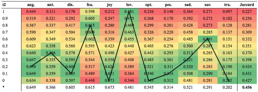
Figures 7 and 8 show the results for the Arabic and English datasets when WCP was used with a
number of fixed thresholds compared to when a varying threshold was allowed, as well as the best
thresholds for each emotion as determined by WCP. It was clear that WCP performed better on some
emotions with higher thresholds and on others with lower thresholds. The “t2” column indicates
the threshold used, followed by the Jaccard score for each emotion at that threshold and the overall
Jaccard score for all the tweets in the last column. The last row in the table shows the best Jaccard
scores for each emotion and the overall Jaccard score. The black line shows the best thresholds for
each emotion. The results for both datasets shared a number of characteristics. WCP selected lower
thresholds for good performance on anger and anticipation. However, for disgust, fear, joy, love and
optimism, the same threshold was selected for the Arabic dataset, whereas for the English dataset,
the thresholds were variable. The last four emotions showed a clear pattern: pessimism and sadness
required low thresholds; surprise needed a threshold higher than both of these; and trust needed a
small threshold for good performance.
Figure 7. Heat-map showing results of different thresholds for the Arabic dataset.
Figure 8. Heat-map showing results of different thresholds for the English dataset.
It is interesting to note the scores at these thresholds (recall that although the thresholds were
important, the aim was to maximise the scores). WCP scored highly for anger at the low thresholds
regardless of the dataset. However, this was the only correlation between the two datasets. For every
other emotion, both datasets behaved differently. Some emotions needed high thresholds, but stillInformation 2019, 10, 98 16 of 20
scored poorly (e.g., surprise in the Arabic dataset); some emotions had low thresholds, but scored poorly
(e.g., trust in the English dataset); some emotions had high thresholds and scored highly (e.g., fear in
the English dataset); and some emotions had low thresholds and scored highly (e.g., pessimism in the
Arabic dataset). This highlights that there were general similarities, but also key differences between
the languages and how they were used to convey emotion in tweets.
For both datasets, WCP performed better at lower thresholds for anger. This reflected the fact that
there were many strong words that were highly indicative of anger alone, e.g., “fuming”, “inflame”,
“pissed”, “scorn”, “furious” and “rage”. Words used to convey anger in the Arabic dataset were,
perhaps, indicative of the current situation in certain Middle Eastern countries: á
JKñmÌ '@ (“Houthis”),
á
JKñmÌ '@ (“irritation”), QºªË@ (“military”), Z@YJ«@ (“assault”). Both sets of words were indicative of anger,
and consequently, obtaining a high score was achieved more easily than for some of the other emotions.
However, at the higher thresholds, the Jaccard score decreased because anger was confused with the
other emotions, e.g., disgust. A small threshold was clearly not the only criteria for a good score, as can
be seen in both datasets, where the best Jaccard for anger was much higher than the best Jaccard for
anticipation, although both had low thresholds. It is interesting to see why the best thresholds were low
for some emotions and high for others.
Higher scoring tokens for an emotion were indicative of strong emotion-bearing words for that
emotion. Tweets that were classified as an emotion due to being strongly indicative towards an
emotion and contained highly emotive words for that emotion remained classified as that emotion,
regardless of the threshold. For example, consider the tweet: “Bloody parking ticket _145__217_#fuming”,
where _145_represents the UNAMUSED FACE emoji and _217_represents the MONEY WITH WINGS
emoji (because this was only used in this one tweet and was removed as a singleton, it had a score of
zero). Due to the presence of “#fuming” and “fume” (and their high scores), the normalised score for
anger was 1.0 (i.e., the largest possible value). Consequently, this tweet was always classified as anger,
regardless of the threshold.
However, this was not always the case, especially for tweets that contained words that were less
emotive or could also be used for other emotions. For example, consider the tweet “brb going to sulk
in bed until friday”. For anger, the tweet only scored 0.177, largely on the basis of the token “sulk”.
Consequently, this tweet would only be classified as anger at the 0 and 0.1 thresholds. Beyond the 0.1
threshold, it would be classified as a false negative for anger, although it may be classified correctly for
some other emotion.
Every emotion had a different optimal threshold; we believe this is due to the fact that different
tokens were important for different emotions and also because there were different numbers of training
tweets for each emotion. If there were more training tweets for trust, for example, there may have been
more words specifically used for trust, and this may have led to more higher scoring tokens for trust.
Every emotion had tokens that scored highly and tokens that scored poorly. However, recall that
for tokens that did not occur in some emotion (e.g., “furious” did not appear in any trust tweets),
these low scores were always large and negative (e.g., −7). For example, recall that trust had the least
number of training tweets. Consequently, for the trust emotion, the lexicon contained relatively few
tokens that genuinely came from trust tweets, but many tokens for trust with large negative scores
that came from other emotions, which would vote against trust. Consequently, according to Figures 7
and 8, for a tweet to be classified as trust, it merely had to achieve a score large enough to exceed the
minimum threshold. Even with this minimal threshold, the Jaccard score for trust was reasonable;
however, this may be due to the small number of test tweets.
The higher the token scores were for an emotion, the more likely that tweets with those tokens
would generate high normalised tweet scores (i.e., closer to the maximum threshold of 1.0). This
made these scores larger than many of the (lower) thresholds, and consequently, the likelihood of
the tweet being classified as that emotion was increased. In other words, emotions containing tokens
with high scores tended to be easier to classify, and the Jaccard scores for these emotions tended to be
higher. However, as seen in the tweet about “sulking in bed until Friday”, not all angry tweets wereInformation 2019, 10, 98 17 of 20
straightforward to classify, and due to these tweets, as the threshold got higher, more and more angry
tweets were classified as false negatives.
Although the final Jaccard scores were similar for both datasets, it is interesting to see that the
emotive words used in the datasets were very different. It was observed that Arabs tend to use
hashtags infrequently in tweets and that many of the top tokens in the Arabic dataset were referring to
the situation in Yemen (“Houthis”, “victory”, “our land”). In general, it was difficult to draw concrete
conclusions from the results because the Arabic dataset was small.
The top Arabic dataset tokens also scored substantially higher than their English counterparts.
It is important to clarify that high scores did not indicate that a token appeared many times in an
emotion or in a dataset, rather it was an indication of the importance of the token to an emotion
relative to the other emotions. Consider the token PAJKB@ (“the victory”). This was the highest scoring
token for trust in the Arabic dataset. However, this token appeared in only five tweets throughout this
dataset, three of which were classified as trust:
“Experience killed mercenaries of Taiz with a weapon and I killed the mercenaries of Twitter. Praise
be to God for these victories. Hehe”
“The feeling of victory”
“Some fans were surprised about the amount of frustration inside them, trust your team and let the
predestination does as it please. Hala Madrid! after defeat comes victory”
The token also appeared twice in tweets classified as optimism. Thus, the probability for the token
was greater for trust than it was for optimism. This difference led to WCP ultimately calculating a high
score for the token for trust. In other words, large scores were generated on the basis of a small number
of tokens; these tokens then went on to contribute over-excessively to tweets being classified as trust.
This step had a reasonable impact on the performance of WCP, since it implicitly weighed up
the likelihood of a given emotion occurring at all, as well as being sensitive to the fact that different
emotions may be expressed in different ways.
Separate thresholds for each emotion increased the overall scores from 0.370 to 0.452 on the Arabic
dataset and from 0.431 to 0.455 on the English dataset.
These results show that this process, while clearly helpful, was not a major contributor to the
difference between WCPs’ performance on the target data and the multi-DNNs’ performance, since the
multi-DNNs also had similar processes. However, the final results on the two datasets were extremely
similar, thus confirming the robustness and adaptability of WCP.
The key elements of WCP, autocorrection and thresholding, showed that with these in place,
significant performance gains were achieved. This is consistent with the initial intuitions that allowing
the algorithm to drop unhelpful words and that a single threshold for all emotions would not be helpful
resulted in significant performance gains. We also observed that certain emotions often presented
together in tweets as pairs. For example, joy and optimism often presented together. We believe that
this also has an effect on the results.
It was noted that WCP performed poorly on the trust emotion. However, only 2% of the tweets
in the datasets were labelled as trust. This was an extremely modest amount of tweets to learn from
and may account for the low scores. However, the surprise emotion had an even smaller number of
tweets, yet WCP managed to perform at least on par with some of the other emotions. This suggested
something different about the tokens used in the trust and the surprise tweets. This difference in
performance may be due to the differences in the numbers of tweets that have multiple emotions.
For example, trust had almost three-times as many tweets that had 2, 3 and 4 emotions than surprise.
It was also noticeable that the English datasets seemed easier to classify.
It is possible that the annotation process also played a part in shaping the results. The crowdsourcing
nature of the annotation left much scope for judgement; hence, datasets constructed in this way are
more difficult to classify due to noise and misclassifications.You can also read