DIAGNOSTIC MEDICAL IMAGING - 3rd Part - Nuclear Magnetic Resonance Imaging
←
→
Page content transcription
If your browser does not render page correctly, please read the page content below
DIAGNOSTIC MEDICAL IMAGING
3rd Part – Nuclear Magnetic Resonance Imaging

          Tommaso Rossi - Modulo di SEGNALI, a.a. 2019/2020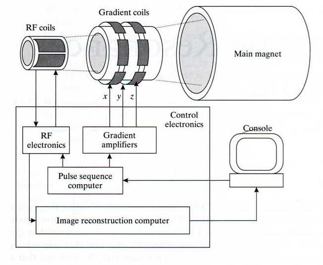
Physics of Magnetic Resonance                                                  2

  Magnetic resonance scanners use the property of nuclear magnetic
  Resonance (NMR) to create images
All nuclei have positive charges (they are composed by protons and
neutrons). A nucleus with either an odd atomic number or an odd mass
number has an angular momentum – they have spin

           The nuclei of the hydrogen atoms (¹H) have spin ½
Rotating charges create an angular magnetic momentum, the rotating
nuclei of the hydrogen atoms similar to little magnets

                      Φ                                                           N

                                                                         +        +
 Nucleus angular                        Microscopic                           +       +
   momentum                            magnetization of                  +
                                          nucleus                         +       +

                                                                                  S

                     Tommaso Rossi - Modulo di SEGNALI, a.a. 2019/2020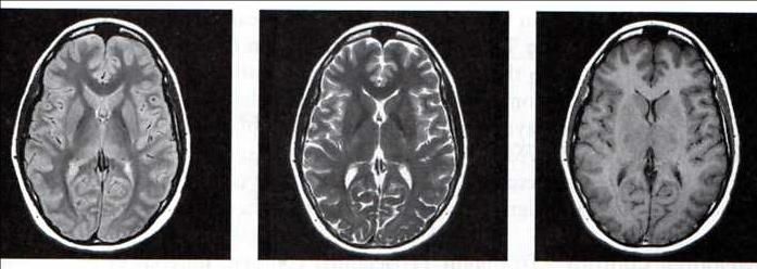
Physics of Magnetic Resonance                                        3

In normal conditions individual spins of ¹H nuclei have a random orientation,
has results no macroscopic magnetic field is produced

If the nuclei of the hydrogen atoms (¹H) are subjected to a strong magnetic
Field, B0 , they tend to align with the field (parallel and anti-parallel
orientation); being the number of hydrogen atoms into the human body
very high, this tendency results in a magnetization of the body

A little more than half of the nuclei will be oriented in the same direction of
the external magnetic field, “up” oreintation (having a lower energy
content), while the others nuclei will be oriented in the opposite direction,
“down” oreintation (having higher energy content).

Random thermodynamic interaction between magnetic dipoles and the
surrounding macro-molecules create a continuous change in spin
orientation. The dynamic difference between “up” and “down” nuclei is
strictly related the external field intensity.

                       Tommaso Rossi - Modulo di SEGNALI, a.a. 2019/2020
Physics of Magnetic Resonance 4
Macroscopic magnetisation grows as B0 grows
A magnetic field of 1.5 T creates a difference between up and down spin
oreintation of 6 p.p.m.
1 mmc of tissue 1019 hydrogen nuclei a significant magnetic
magnetisation is produced
Actually, nuclei spin precess around an axis along the direction of the
field. This precession has a frequency, called Larmor frequency
(proportional to B0 ), of the order of MHz (radiofrequency).
As an example the precession
frequency for an external field of
1.5 T is 64 MHz B0
Tommaso Rossi - Modulo di SEGNALI, a.a. 2019/2020Macroscopic Magnetisation 5
It i simportant to underline that there is no precession phase coherence
between nuclei z
The xy plane components of the
microscopic magnetisation vectors are
placed in every directions, their sum is LMM0≠0
zero. This component of the macroscopic
magnetisation is called Transversal
x y
Macroscopic Magnetisation TMM0=0
The z plane components of the
microscopic magnetisation vectors are
placed both in z and –z directions.
Their sum is positive along z direction.
This component of the macroscopic
magnetisation is called Longitudinal TMM0=0
y
Macroscopic Magnetisation LMM0≠0
x
Tommaso Rossi - Modulo di SEGNALI, a.a. 2019/2020Macroscopic Magnetisation 6
The Macroscopic Magnetisation produced by the external magnetic
field is static and smaller than B0 it is not possible to measure it
An external excitation has to be introduced in the system
If a microscopic sample of nuclei is excited using a electromagnetic
radiation having Larmor frequency, the radiation magnetic component
interacts with nuclei magnetic moment
A quantum of energy is absorbed changing the nuclei energy status
from “up” to “down”
The longer is the RF pulse duration the higher is the energy transfered
to the system (the higher is the number of nuclei that changes their
status from up to down)
When these energy transitions occur, nuclei are resonant with applied
radiation
The Bloch equations are a set of coupled differential equations which
can be used to describe the behavior of a MM vector
Tommaso Rossi - Modulo di SEGNALI, a.a. 2019/2020Macroscopic Magnetisation 7
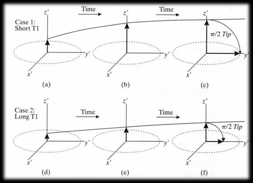
When the difference between up and down spin populations decreases
their precession phase syncronisation grows
It is possible to set the RF pulse duration to reach the condition of
having the same “up” and “down” spin population that have complete
precession phase coherence This RF is called “90° Pulse”
The system subject to the 90° Pulse has LMM1=0 while the TMM1 reach
its maximum, the TMM rotate in the xy plane with the nuclei precession
frequency (the RF pulse one)
z
The MM, following a spiral movement
with growing ray, deflects from its
position along z axis to a position in
the xy plane, so it is rotated by 90°
TMM1 growing
x y
y
x LMM1 decreasing
Tommaso Rossi - Modulo di SEGNALI, a.a. 2019/2020Macroscopic Magnetisation 8
If the duration of the RF pulse is doubled (w.r.t. the one of the 90° pulse)
It is possible to obtain the total “up” and “down” populations reversal
(w.r.t. the initial situation), in this status there is no precession phase
coherence between nuclei LMM2= -LMM0 , TMM2=0
This RF is called “180° Pulse”
It is clear that it is possible to change RF pulse amplitude and duration
so that different degrees of deflection of MM can be obtained
The displacement of MM from its longitudinal direction leads to a
unstable system (no energetic equilibrium), having high energy and
high phase nuclear synchronisation
When the external RF ends the system goes back to initial conditions
Tommaso Rossi - Modulo di SEGNALI, a.a. 2019/2020Relaxation 9
When the external RF ends, the rapidly rotating (and decreasing) TMM
creates a radio frequency excitation within the sample that will in turn
induce (Faraday induction) a voltage in a coil of wire located outside the
sample. This signal is recorded for use in MRI.
Transverse relaxation, also known as spin-spin relaxation, acts first to
cause this received signal to decay. This relaxation is caused by the
perturbations in the magnetic field due to other spins that are nearby.
This interaction causes spins to momentarily speed up or slow down,
changing their phases relative to other nearby spins (dephasing).
The resulting signal is called free induction decay (FID),
an exponential decay having a time constant called
transverse relaxation time, T2
Tommaso Rossi - Modulo di SEGNALI, a.a. 2019/2020Free Induction Decay 10
FID amplitude is a function of the number of nuclei in the sample,
the decreasing time is a function of the decreasing speed of TMM
It is not easy to botain a good FID sampling, due to the fact that the
transmitting and receiving coils are the same, moreover the FID
signal decreases very quickly and is effected by non homogeneous
magnetic field of the structure
The RF pulses practically used in NMR imaging create spin echoes
Tommaso Rossi - Modulo di SEGNALI, a.a. 2019/2020Relaxation 11
T2 is the time required to the TMM to reach the 37% of its initial value
(reached when the RF pulse is applied)
There are two factors causing the decreasing of phase coherence of
resonant nuclei
-The energy transitions of nuclei that changes their status from down to
up
- Interactions between spin and molecular micro-EM field, these
interactions do not vary the energy of the system but create local
variations of the static field, B0 ,inducing a change in precession velocity
(phase displacement)
Actually, local perturbations of B0 cause the received signal to decay
exponentially with a time constant T2*, lower than T2
This effect is reversible using the technique of coherence refocusing
thorugh the concept of echoes (that will be described later)
Tommaso Rossi - Modulo di SEGNALI, a.a. 2019/2020Relaxation 12
The second relaxation mechanism is called longitudinal relaxation or
spin-lattice relaxation.This process concerns the longitudinal
magnetisation which recovers back to its equilibrium value as a rising
exponential having a time constant called longitudinal relaxation time, T1
T1 is the time required to the LMM to reach the 63% of its equilibrium value
T1 is a function of how fast the spin systems release energy to return from
down to up position, this thermodynamic energy exchange involves the
surrounding molecules (this process is a function of B0 )
T1 and T2 are different for various types of tissues and are responsible for
generating contrast in MR images. For tissue in the body the relaxation
times are in the ranges: 250 ms ≤ T1 ≤ 2500 ms , 25 ms ≤ T2 ≤ 250 ms
Usually 5T2 ≤ T1 ≤ 10T2 and for all materials T2 ≤ T1
This is due to the fact that there are spin-spin interactions that cause
phase coherence loss without changing up and down populations,
therefore T1 relaxation gives contribution to T2 relaxation but not vice-versa
Tommaso Rossi - Modulo di SEGNALI, a.a. 2019/2020Relaxation 13
Mz = Mo ( 1 - e-t/T1 ) MXY =MXYo e-t/T2
Tommaso Rossi - Modulo di SEGNALI, a.a. 2019/2020Relaxation 14
Proton density, PD, is the number of resonant nuclei per unit volume.
The greater is PD the greater is the relaxation signal intensity
It has to be outlined that not all the hydrogen nuclei in the tissues will
give contribution to the MR signal, just the resonant ones (in particular
the ones that are in “free water”).
Solid structures that are made of a great number of nuclei, as bones,
have a little percentage of mobile resonant nuclei therefore the MR
signal is very low.
Larmor frequency is a function of the applied magnetic field but it is also
influenced by the electron clouds surrounding the nuclei that creates a
small local EM field that ineracts with B0
Chemical shift is the variation of the resonance frequency in different
substrates that is a function of the shielding effect produced by atom
electrons on B0
Tommaso Rossi - Modulo di SEGNALI, a.a. 2019/2020Pulse Sequences 15
Generation of Spin Echoes: when the RF 90° pulse ends spins begin to point
in different directions in the transverse plane, therefore there are “faster”
and “slower” spins.
If a RF 180° pulse is applied to
the system the spin directions in
the transverse plane is inverted
and from this new position the
fast spins “catch up” and the
slow spins “fall back”.
Therefore the signal generated by
transverse spins recovering their
coherence creates a spin echo
that can be easily measured.
The time interval from the initial 90° pulse to the formation of the spin echo
is called echo time TE, the application time of the 180° pulse is TE/2
Tommaso Rossi - Modulo di SEGNALI, a.a. 2019/2020Pulse Sequences 16 Generation of Spin Echoes Tommaso Rossi - Modulo di SEGNALI, a.a. 2019/2020
Contrast Mechanism                                     17

In MRI the ability to generate tissue contrast depends on both the intrinsic
MNR properties of the tissue (PD, T1, T2) and the characteristics of the
externally applied excitations.

It is possible to control the tip angle, the echo time, TE, of the RF
excitation and the pulse repetition interval, TR.

This does not means that the brightness of the images are proportional
to one of the three parameters but merely that the differences in intensity
seen between different tisuses are largely determined by the difference in
one of the three parameters

             Three time of weighted contrast can be used:
             • PD-weighted
             • T1-weighted
             • T2-weighted
                        Tommaso Rossi - Modulo di SEGNALI, a.a. 2019/2020
Contrast Mechanism 18
PD-weighted T2-weighted T1-weighted
Tissue Type Relative PD T2 (ms) T1 (ms)
White matter 0.61 67 510
Grey matter 0.69 77 760
Cerebrospinal fluid 1.00 280 2650
Tommaso Rossi - Modulo di SEGNALI, a.a. 2019/2020Contrast Mechanism 19
T1-weighted contrast: the image intensity should be proportional to T1.
The differences in the longitudinal component of magnetisation must
be emphasized.
Short TE and TR has to be used. Short TE allows to image the echo signal
when the phase coherence loss, dependant on T2, is small (so that the
differences between tissues that are a function of T2 are minimised).
Short TR, lower than the one of the tissue being imaged, allows the
measured signal to be dependant on the LMM recovery time, i.e. short T1
tissues give rise to stronger signals.
Usually TR is shorter than the T1 of the tissues having long T1 and of
the order of T1 of the tissues having short T1. Intensity of tissues
having long T1 will be very low (dark-gray colours), tissues having
short T1 will look very bright (white-gray colours).
In the brain-slice picture TR=600 ms, TE=17 ms and tip angle is 90°
Tommaso Rossi - Modulo di SEGNALI, a.a. 2019/2020Contrast Mechanism 20
T1-weighted contrast
Image
Tommaso Rossi - Modulo di SEGNALI, a.a. 2019/2020Contrast Mechanism 21
T2-weighted contrast: the image intensity should be proportional to T2.
Differences in the transverse relaxation times of different tissues must be
apparent.
Long TE and TR has to be used. Long TE allows to image the echo signal
when the phase coherence loss is high (so that the differences between
tissues that are a function of T2 are maximised).
Long TR, greater than the T1 of the tissue being imaged, allows the
measured signal to be not dependant on the LMM recovery time, so that
the T1 differences between tissues are very negligible.
For tissues having long T2, as fluids, the duration of phase cohernece is
very high, so if the signal is analysed after a long TE the echoes
intensity is still high.
Intensity of tissues having short T2 will be very low (dark-gray colours),
tissues having long T2 will look very bright (white-gray colours).
In the brain-slice picture TR=6000 ms, TE=102 ms and tip angle is 90°.
This value of TR is practically not usable because the images take too
long to acquire.
Tommaso Rossi - Modulo di SEGNALI, a.a. 2019/2020Contrast Mechanism 22
PD-weighted contrast: the image intensity should be proportional to the
number of resonant hydrogen nuclei in the sample.
Short TE and long TR has to be used.
Starting form the sample in equilibrium a excitation RF pulse is applied
then, before the signal has a chance to decay from T2 effects, the
relaxation signal has to be imaged quickly. Therefore long TR (which
allows the tissues to be in equilibrium, no dependance on T1) and either
no echo or short TE (in order to minimize dependence from T2 decay) has
to be used.
The preferred tip angle is 90°, to obtain maximum signal.
Intensity of tissues having low PD will be very low (dark-gray colours),
tissues having high PD will look very bright (white-gray colours).
In the brain-slice picture TR=6000 ms, TE=17 ms and tip angle is 90°.
This value of TR is practically not usable because the images take too
long to acquire.
Tommaso Rossi - Modulo di SEGNALI, a.a. 2019/2020MRI Scanner 23
An MRI scanner consist of five principal components:
• The main magnet
• A set of switchable gradient coils
• RF coils
• Pulse-sequence end receive
elctronics, used to program timing
of transmission and reception of
signals
• Console for viewing, manipulating
and storing images.
Tommaso Rossi - Modulo di SEGNALI, a.a. 2019/2020MRI Scanner 24
The main magnet is commonly a cylindrical superconducting magnet
having field strength ranging from 0.5 to 7 T
The gradient coils produce the change in local magnetic field
necessary to encode the spatial location of the MR signal (this will be
discussed later)
The RF coils, or resonators, both induce
the RF signals to tip the magnetisation
vector and have current induced in them
by the spin systems. Therefore RF coils
are used for the transmission and
reception of RF pulses.
Tommaso Rossi - Modulo di SEGNALI, a.a. 2019/2020Image Formation 25
How can we encode spatial position of MR signals?
An MR scanner can create images at arbitrary location and orientation,
for simplicity, the formation af axial images will be discussed
The MR signal contributions coming from different voxels is obtained
through the use of magnetic field gradients and the spatial position is
encoded using frequency and phase (of the signal)
Lets apply a field gradient on the x-axis to the external field.
Due to the fact that the spin precession frequency is directly proportional
to the field, the sample spins will be characterised by different precession
velocities (along x-axis)
Tommaso Rossi - Modulo di SEGNALI, a.a. 2019/2020Image Formation 26
Lets consider 8 water
samples, and a External field intensity MR signal intensity
magnetic field that
crosses the samples
Static B, the MR signal
frequency is concentrated
x axis Frequency
If a gradient is applied, the External field intensity MR signal intensity
MR signal frequency
analysis can be used to
identify the sum of the
voxels signals along the
planes perpendicular to
the gradient
x axis Frequency
Tommaso Rossi - Modulo di SEGNALI, a.a. 2019/2020Slice Selection 27
In CT and ultrasound the energy used to
image the selected slice is restricted to the
slice itself, there is no other part of the body
from which signal can arise.
In SPECT and PET the whole body is a
potential source but the observed signal is
selected by collimation so that it belongs to a
specific slice.
In MRI both these approaches can be used, it
is possible to excite only a selected slice or it
is possible to excite the entire volume and
then to extract images of selected slice.
The first technique is called 2-D MR imaging, the second is called 3-D
MR imaging.
Only the first technique will be analysed.
Tommaso Rossi - Modulo di SEGNALI, a.a. 2019/2020Slice Selection 28
A magnetic field gradient along z-axis,
High Gradient
called selection gradient, is used to
select the slice to be imaged
The higher is the gradient the Low Gradient
thinner is the slice, considering RF pulse
a fixed bandwidth of the RF bandwidth
pulse
The RF pulse is a sinc function
that has a rectangular Fourier
transform able to excite a range
of frequencies which in turn
High Gradient
excites a range of tissues layer selection
Low Gradient
layer selection
Tommaso Rossi - Modulo di SEGNALI, a.a. 2019/2020“Projection and Reconstruction” Method 29
Once the slice is selected another gradient has to be applied in order to
encode the spatial position of the MR signal.
This new gradient has a different position w.r.t. the selection gradient and
it is located along x-axis and it is called readout gradient.
The first storical method used to lacate MR signal is called projection and
reconstruction
After the application of the selection gradient, an echo signal is created
through the use of a 90° RF pulse followed by a 180° RF pulse.
During the creation and for all the duration of the echo a readout gradient
is applied, for example along x-axis, so that it is possible to discriminate
in the frequency domain the contributions coming from different “strips”
perpendicular to x.
A “projection” of the selected slice along x-axis is obtained.
In order to reconstruct the image multiple projections have to be
created.
Tommaso Rossi - Modulo di SEGNALI, a.a. 2019/2020“Projection and Reconstruction” Method 30
Different projections can be obtained in the same way described before
but applying a combination of readout gradients along x-axis and y-axis
so that to obtain different gradients along xy-plane
A number of equally spaced projections between 0° and 180° are
acquired
The collected data are processed using one of the methods used to
reconstruct CT images:
• Forurier Method
• Filtered Backprojection
• Convolution Backprojection
From the MR signals it is possible to obtain a map of multiple
parameters, PD, T1 and T2
Tommaso Rossi - Modulo di SEGNALI, a.a. 2019/2020“Projection and Reconstruction” Method 31
Monodimensional
projection, having an
Amplitude
Slice selection, angle defined by Gx
through Gz and RF and Gy
Frequency
Nuclear signal echo echo
Tommaso Rossi - Modulo di SEGNALI, a.a. 2019/20202D DFT Method 32
In order to decrease the computational complexity the image
reconstruction based on the bidimensional Fourier transform is used.
For this method a series of projections is requested in order to
reconstruct the image.
After the application of the selection gradient, an echo signal is created
through the use of a 90° RF pulse followed by a 180° RF pulse.
During the creation and for all the duration of the echo a fixed readout
gradient along x-axis is applied (the readout gradient is the same for
every projection).
The signal position is coded using for every projection a different Gy,
applied right after the 90° pulse and before the 180° pulse in order to
create a spin dephasing (along xy-plane) that is a function of the position
along the y-axis of the element that generated the signal.
Tommaso Rossi - Modulo di SEGNALI, a.a. 2019/20202D DFT Method 33
No gradient: Gradient on: Gradient of:
spin in phase spin dephasing final phase
remembered
Gy
time
y0
Tommaso Rossi - Modulo di SEGNALI, a.a. 2019/20202D DFT Method 34
If a Gy gradient is applied before the creation of the echo the nuclei
located in a position with higher y coordinate precess faster than the
ones having lower y coordinate.
When the Gy gradient ends all the nuclei start precess at the same
velocity. So it has been created a dephasing that is a function of the
position along the y-axis.
After the 180° pulse an echo rise up. Afterwards the Gx gradient is
applied in order to change the precession frequency of the spins as a
function of their position along x-axis, but these spins will maintain the
dephasing acquired during the application of the Gy gradient that codes
their position along y-axis. The Gy gradient is called phase encoding
gradient.
The Gz gradient select the slice while phase and frequency of the
measured signal reflect its postion along y and x axes respectively
Tommaso Rossi - Modulo di SEGNALI, a.a. 2019/20202D DFT Method 35
One monodimensional
projection along x
direction having phases
Amplitude
Amplitude
coded by Gy
Slice selection,
through Gz and RF
Frequency Frequency
echo echo
Nuclear signal
Tommaso Rossi - Modulo di SEGNALI, a.a. 2019/202036
Example (1/5)
Phase
We record the phase change at change at
the top of the knee during the the top of
phase encoding process the knee
phase encoding
Rate of change
each K-Space
of phase
signal is
from the
whole
knee
frequency encoding
We started with a large positive phase change,
and ended up with a large negative phase change.
Over all the phase encoding steps, we have a rate
of change of phase = frequency
Tommaso Rossi - Modulo di SEGNALI, a.a. 2019/202037
Example (2/5)
Phase change
We record the phase change for for the section
another section of the knee during of the knee
the phase encoding process
phase encoding
Rate of change
each K-Space
of phase
signal is
from the
whole
knee
frequency encoding
We started with a medium positive phase change,
and ended up with a medium negative phase
change. Over all the phase encoding steps, we
have a rate of change of phase = frequency
Tommaso Rossi - Modulo di SEGNALI, a.a. 2019/202038
Example (3/5)
No phase
We record the phase change for the change for the
central section of the knee during the central section
phase encoding process of the knee!
phase encoding
each K-Space
signal is
from the
whole
knee
frequency encoding
During the phase encoding of the central section of
the knee, the Gy phase encoding gradient is zero!
Tommaso Rossi - Modulo di SEGNALI, a.a. 2019/202039
Example (4/5)
Phase change
We record the phase change for for the section
another section of the knee during of the knee
the phase encoding process
phase encoding
Rate of change
each K-Space
of phase
signal is
from the
whole
knee
frequency encoding
We started with a medium negative phase change,
and ended up with a medium positive phase
change. Over all the phase encoding steps, we
have a rate of change of phase = frequency
Tommaso Rossi - Modulo di SEGNALI, a.a. 2019/202040
Example (5/5)
Phase change
We record the phase change for for the bottom
the bottom of the knee during the of the knee
phase encoding process
phase encoding
Rate of change
each K-Space
of phase
signal is
from the
whole
knee
frequency encoding
We started with a large negative phase change, and ended up with a large positive
phase change. The Fourier transform can separate out different frequencies (even ones
that are made from a rate-of-change of phase over many phase encoding steps), we
now have a way of determining the total signal from each of the rows!
Tommaso Rossi - Modulo di SEGNALI, a.a. 2019/20202D DFT Method 41
All the acquired data are stored in the so called K-space
Each row of the K-space is a monodimensional projection data; then, in
order to reconstruct the image a bidimensional DFT is applied to the K-
space
The first DFT is applied to all the rows obtaining information on intensity
of the frequency components and on their phases
The second DFT is applied to all the columns obtaining information on the
RM signal charcateristics
This method is preferred with respect to the Projection and
Reconstruction one due to the fact that is more efficient w.r.t.
computational complexity; in fact FFT can be used to reduce complexity.
Tommaso Rossi - Modulo di SEGNALI, a.a. 2019/20202D DFT Method 42
Two voxels having
different magnetization Raw Data
Two oscillations frequencies in the
time domain & two oscillation
frequencies in the phase domain
Tommaso Rossi - Modulo di SEGNALI, a.a. 2019/20202D DFT Method 43
FFT in the frequency FFT in the phase
encoding direction encoding direction
Oscillations in the
phase encoding
direction
Tommaso Rossi - Modulo di SEGNALI, a.a. 2019/2020MR Image Quality 44
MR image quality is affected by intrinsic and extrinsic factors
Intrinsic factors are a function of the examined tissues and affect signal
Intensity, these factors are:
Proton density, Spin-spin relaxation time, Spin-lattice relaxation time,
Chemical shift, Movement, Temperature.
Extrinsic factors are a function of the scanner, the installation site,
environment and patient, these factors affect contrast and spatial
resolution.
Contrast is essentially a function of RF sequence, as previously
explained, and external magnetic field intensity.
Spatial resolution is a function of magnetic field homogeneity and
gradients linearity; these two factors optimize the spatial location of
the signal. Also RF Tx-Rx equipments affect spatial resolution.
Moreover spatial resolution grows as pixel dimensions and slice
tickness decrease and as signal to noise ratio, S/N, grows.
Tommaso Rossi - Modulo di SEGNALI, a.a. 2019/2020You can also read