DigitalCommons@USU Utah State University
←
→
Page content transcription
If your browser does not render page correctly, please read the page content below
Utah State University
DigitalCommons@USU

Physics Capstone Projects                                                   Physics Student Research

5-2-2022

Seasonal Variations in Global Ionospheric Total Electron Content
Jason Knudsen
Utah State University

Follow this and additional works at: https://digitalcommons.usu.edu/phys_capstoneproject

    Part of the Physics Commons

Recommended Citation
Knudsen, Jason, "Seasonal Variations in Global Ionospheric Total Electron Content" (2022). Physics
Capstone Projects. Paper 103.
https://digitalcommons.usu.edu/phys_capstoneproject/103

This Article is brought to you for free and open access by
the Physics Student Research at DigitalCommons@USU.
It has been accepted for inclusion in Physics Capstone
Projects by an authorized administrator of
DigitalCommons@USU. For more information, please
contact digitalcommons@usu.edu.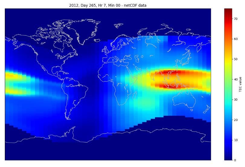
Seasonal Variations in Global Ionospheric Total Electron Content
         Jason Knudsen

         Physics 4900 Research in Physics

         Department of Physics, Utah State University, Logan, Utah

As the Sun ionizes atoms and molecules in the Earth’s ionosphere, the region of atmosphere above approximately 100
km in altitude, the created ionization in this region affects many of the systems that we rely on in daily life. This
includes cellular service, GPS navigation, weather forecasting, and credit card data. A good measure for the level of
ionization in the ionosphere is total electron content (TEC), which is the number of electrons in a square column above
a given geographic location. The TEC over a geographic location influences the propagation of radio waves that
traverse that section of the ionosphere. With severe enough conditions, radio waves sent through the ionosphere can
become corrupt or read back with significant levels of inaccuracy. Thus, monitoring and modeling TEC patterns and
variations allows us to better understand and prepare for the constantly changing ionosphere. TEC data is gathered
from thousands of ground-based GPS receivers around the globe, and TEC distributions between seasons can be
compared to each other. Data analysis showed qualitative trends relating the spring and fall equinoxes as well as the
summer and winter solstices.

         Report submitted: May 2, 2022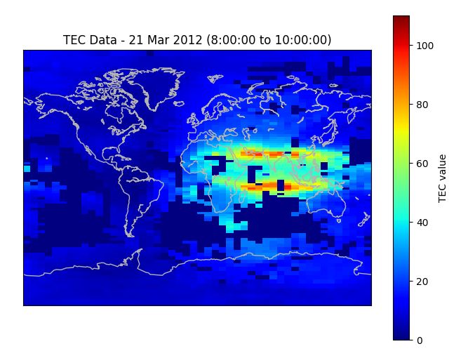
Introduction

The term “space weather” is a broad term that describes the numerous ways in which variations in
which solar electromagnetic and charged particle emissions influence the Earth’s atmospheric and
environmental systems. The ionosphere, the region of the Earth’s atmosphere starting at around
80 to 100 km in altitude, constantly experiences changing space weather as a result of the
constantly changing conditions of the Sun [1]. While solar emissions are the primary driving force
in space weather and its variations, lower atmospheric disturbances can also add a nontrivial
amount of variability seen in this region [2].

As many of our daily services increasingly rely on sending radio waves through the ionosphere to
satellites in low orbit, understanding space weather becomes increasingly vital to human function
and activity. Many of the most commonly used digital applications, including cellular service,
Global Positioning System (GPS) navigation, and credit card transactions, all rely on sending radio
waves through the ionosphere to and from satellites and are thus directly impacted by space
weather [1-2]. If conditions are too severe, these signals can become distorted, rendering the data
contained within the signals unreliable. In addition, severe space weather conditions can have
impacts on other human functions, including power grids and pipeline infrastructures. In the worst
cases, potentially catastrophic scenarios such as power outages and blackouts can be caused as a
direct result of sufficiently extreme space weather conditions [1].

Therefore, it is crucial that space weather conditions are constantly monitored. One good measure
of ionospheric activity is total electron content (TEC), the number of electrons in a square column
above a given area. TEC distributions are under constant flux, and distributions will appreciably
vary by the day and even by the hour [2]. As the Sun is the primary driving force behind space
weather phenomena, it also naturally follows that seasonal variations in TEC will occur. By
comparing TEC distributions from various times of day and year, patterns begin to emerge, and
comparative observations can be made. This report details the research on seasonal TEC variations
in the year 2012, and was conducted over the Fall 2021 and Spring 2022 semesters.

Methods

Every five minutes, thousands of ground-based GPS receivers across the globe monitor the
ionosphere and take TEC readings in the region immediately above their respective locations.

                                                 1
Sensors in each geographic region detect vast numbers of electrons at a time (on the order of 1016).
Thus, to allow the TEC data to be human readable, the actual number of detected electrons in each
reading is stored in data files after dividing the observed TEC count by a factor of 1016. This
transforms each TEC data point onto a clean number that falls into a range of approximately 0 to
110. The receivers also save pertinent locational and time information that detail when and where
each TEC measurement took place. Parameters including longitude and latitude coordinates,
altitude measurements, and the time of data collection (in UT time) all accompany each TEC data
point. Thus, each logged set of data also has associated date, time, and locational information
attached to all points within each set.
As the thousands of GPS receivers each take nearly three hundred measurements throughout a
single day, data sets are organized into separate data files for each day. However, due to the sheer
size and number of data points per file, raw data files are impossible to analyze without computer
assistance. Thus, a program to generate a visualization of the overall distribution of a data set in
question had to be generated over the course of the research. The files containing all data sets
pertinent to this research was retrieved from the Madrigal Database.
Python was chosen as the programming language to interpret and visualize TEC data. Programs to
organize TEC data within each data set based on time increments and programs to generate
visualize data distributions were then written. Once these programs were written, TEC
distributions from different times of day and year were compared to each other. As was discussed
above, the Sun is the primary driver behind space weather phenomena (and thereby TEC
distributions), and this naturally leads to variations in distributions across day and night cycles as
well as across yearly seasonal cycles. Thus, data collected all day during the spring and fall
equinoxes and the summer and winter solstices were retrieved from the Madrigal Database for
comparison and examined via the aforementioned Python programs.
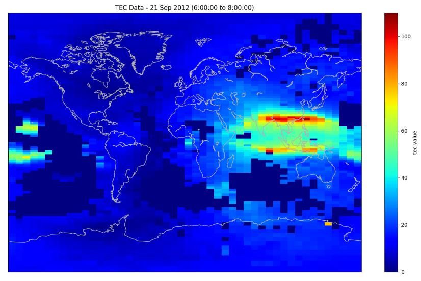
The output of the data visualization programs was generated in the form of sets of twelve color
maps that depicted global TEC distributions in 2 hour increments across each day. Figure 1 below
shows the heat map for the 8:00 to 10:00 UT frame of the 2012 fall equinox. Note that since the
GPS receivers used to collect the TEC data used in the distribution are all ground-based, there are
a large number of regions where data collection is not possible, since the presence of an island or
2landmass upon which to set up the receiver is necessary to collect data from that region. Thus,
many of the regions above oceans and other bodies of water show no TEC information.
Figure 1 – The generated TEC color map from 8:00 to 10:00 UT during the 2012 spring equinox. The two
regions over Southeast Asia with the highest TEC counts are located approximately 15 latitudinal degrees north
and south of the Earth’s magnetic equator, and is collectively known as the equatorial ionization anomaly [3].
By generating several color maps from the 2012 equinoxes and solstices, seasonal comparisons of
TEC distributions and data were able to be made. The results section below explains in detail the
observations and findings from these comparisons.
In addition to raw TEC distributions, servers on Utah State University (USU) campus run physics-
based ionosphere models to help specify space weather conditions to agencies that rely on space
weather data and reports. Models for the 2012 equinoxes and solstices were retrieved, and were
subsequently visualized using similar Python programs to those used in the data organization and
visualization used for the observed TEC data. These model visualizations were then compared to
the TEC data visualizations to observe similarities between the two. In addition, since the physics-
based models do not rely solely on ground-based receivers, they show data and distributions for
regions that the ground-based GPS receivers do not. Thus, the model also provides insights as to
what TEC distributions look like in regions where no GPS receiver was present.
3Results
By comparing global TEC distributions across spring, summer, winter, and fall 2012, some
qualitative trends emerged from the data. For instance, the highest recorded TEC values for each
equinox and solstice always occurred between 6:00 and 10:00 UT, and were always located over
India and Southeast Asia. In addition, the TEC during spring and fall was consistently higher than
the TEC during the summer and winter. The table below shows TEC high point data for each of
the solstices and equinoxes for the year 2012.
Date (2012) TEC High Time (UT) Location
Spring Equinox 109 6:00 to 8:00 S.E. Asia
Summer Solstice 78 6:00 to 8:00 S.E. Asia
Fall Equinox 107 6:00 to 10:00 S.E. Asia
Winter Solstice 66 6:00 to 10:00 S.E. Asia
Various observations regarding overall TEC distributions in each season were able to be seen as
well. During the spring and fall equinoxes, space weather activity was generally confined to the
lower latitudes in the equatorial regions. During the summer and winter solstices, however, most
of the activity was seen across larger geographic regions, and was not mainly confined to lower
latitudes. More specifically, the summer solstice saw significant space weather activity across the
entirety of the northern hemisphere, and the winter solstice saw significant space weather activity
across the entirety of the southern hemisphere.
In addition to overall distributions, local regions of elevated TEC were also visible in the seasonal
color maps. Such regions are known as “anomalies,” and depending on the season, various
anomalies became more or less visible. For example, during the fall equinox, an anomaly off the
southeastern coast of Africa is very visible. However, during the other seasons of the year, this
anomaly becomes far less visible. Another anomaly off the southern coast of South America
(known as the “Weddell Sea Anomaly”) is the most visible during the winter solstice. It can be
seen to a lesser degree during the summer solstice, and becomes even less so during the fall and
spring equinoxes.
4The physics-based ionosphere models were very beneficial to look at as well. Figure 2 below
shows a side-by-side comparison of a model output from the 2012 fall equinox and the collected
data distribution from the same day. The TEC distributions in both maps are very similar, and the
anomaly off the southeastern coast of Africa is shown very clearly in the model output. In addition,
data for the regions where TEC observations were not possible are present in the model output.
This allows for inferences to be made as to what the TEC observations would have looked like for
those specific areas had it been possible to establish a receiver in the area.
Figure 2 – A physics-based ionosphere model output for the 2012 fall equinox (left) and the corresponding
observed TEC data from the same day (right). Note the general shape of each distribution, and the visible
anomaly off the southeastern coast of Africa in both maps.
Conclusions
A variety of individual factors contribute to overall TEC distributions and variations, including
solar activity, wind strength and direction, electric fields, and lower atmospheric disturbances. For
example, the systematically higher levels of TEC over Southeast Asia are believed to be the result
of elevated lower atmospheric activity influencing ionospheric conditions, including local storm
and wind conditions.
The seasonal variations in which the regions where space weather activity was the highest is
believed to be the result of the relative locations of the Earth’s poles and hemispheres with respect
to the Sun at different times of year. Due to tilt in the Earth’s spin axis, the Earth’s geographic
north pole points toward the Sun during the summer solstice, which corresponds to the northern
hemisphere exhibiting the greatest amount of space weather activity during that time. During the
5winter solstice, the Earth’s geographic south pole points towards the Sun, which corresponds to
the southern hemisphere exhibiting the greatest amount of space weather activity during that time.
And finally, during the spring and fall equinoxes, the Earth’s geographic north and south poles are
equidistant from the Sun, which corresponds to the equatorial region (the region exactly in between
the north and south poles) exhibiting the greatest amount of space weather activity during that
time.
By collecting space weather data (including TEC) constantly throughout the year, model results
like the one seen above in Figure 2 can be used to specify space weather conditions. These in turn
help ensure that the systems that rely on transmitting information through the ionosphere continue
to function properly and accurately. As our ability to monitor and predict variations in space
weather continue to improve, so will our capacity to prepare for extreme conditions that have the
ability to adversely impact the systems that we so heavily rely on.
6References
[1] M. Moldwin, An Introduction to Space Weather. (Cambridge University Press, New York,
2008).
[2] R. W. Schunk, L. Scherliess, J. J. Sojka, “Recent approaches to modeling space weather,” Adv.
Space Res., 31, 819 (2003).
[3] B. Zhao et al., “Characteristics of the ionospheric total electron content of the equatorial
ionization anomaly in the Asian-Australian region during 1996–2004,” Ann. Geophys., 27, 3861
(2009).
7You can also read