DIRAC MATERIALS FOR SUB-MEV DARK MATTER DETECTION: NEW TARGETS AND IMPROVED FORMALISM
←
→
Page content transcription
If your browser does not render page correctly, please read the page content below
Dirac Materials for Sub-MeV Dark Matter Detection: New Targets
                                                               and Improved Formalism
                                                         R. Matthias Geilhufe1 , Felix Kahlhoefer2 and Martin Wolfgang Winkler3
                                           1    Nordita, KTH Royal Institute of Technology and Stockholm University, Roslagstullsbacken 23,
                                                                                    10691 Stockholm, Sweden
                                               2 Institute for Theoretical Particle Physics and Cosmology (TTK), RWTH Aachen University,

                                                                                   D-52056 Aachen, Germany
                                                   3 The Oskar Klein Centre for Cosmoparticle Physics, Department of Physics, Stockholm

                                                                       University, Alba Nova, 10691 Stockholm, Sweden
arXiv:1910.02091v2 [hep-ph] 27 Feb 2020

                                                                                             Abstract

                                                      Because of their tiny band gaps Dirac materials promise to improve the sensitivity for dark
                                                  matter particles in the sub-MeV mass range by many orders of magnitude. Here we study several
                                                  candidate materials and calculate the expected rates for dark matter scattering via light and
                                                  heavy dark photons as well as for dark photon absorption. A particular emphasis is placed on
                                                  how to distinguish a dark matter signal from background by searching for the characteristic daily
                                                  modulation of the signal, which arises from the directional sensitivity of anisotropic materials
                                                  in combination with the rotation of the Earth. We revisit and improve previous calculations
                                                  and propose two new candidate Dirac materials: BNQ-TTF and Yb3 PbO. We perform detailed
                                                  calculations of the band structures of these materials and of ZrTe5 based on density functional
                                                  theory and determine the band gap, the Fermi velocities and the dielectric tensor. We show
                                                  that in both ZrTe5 and BNQ-TTF the amplitude of the daily modulation can be larger than
                                                  10% of the total rate, allowing to probe the preferred regions of parameter space even in the
                                                  presence of sizeable backgrounds. BNQ-TTF is found to be particularly sensitive to small dark
                                                  matter masses (below 100 keV for scattering and below 50 meV for absorption), while Yb3 PbO
                                                  performs best for heavier particles.

                                          1      Introduction
                                          The realization that quantum materials, which have been the subject of great attention in recent
                                          years, may offer unique opportunities to search for light and very weakly interacting particles has led
                                          to a fruitful collaboration between particle physics and condensed matter physics. This development
                                          has given new hope to the ongoing search for dark matter (DM) in a time when experimental null
                                          results mount increasing pressure on traditional DM models (see e.g. [1]). Indeed, many novel
                                          detection strategies have been developed that promise to probe DM models in regions of parameter
                                          space that were previously thought to be experimentally inaccessible [2, 3]. This is especially true
                                          for DM particles with mass in the keV to MeV range, which would carry so little kinetic energy
                                          in the present Universe that their interactions with conventional detectors would be unobservable.
                                          While such particles are too light to be produced via the conventional freeze-out mechanism, recent
                                          studies have explored many alternative ways to reproduce the observed DM relic abundance, for
                                          example via the freeze-in mechanism [4–10].

                                                                                                 1
Given the typical velocity of DM particles in the solar neighborhood of v = 10−3 c, one needs to
achieve an energy threshold of less than an eV in order to search for DM particles in the sub-MeV
range. Among the proposed materials to achieve this goal are superconductors [11–13], superflu-
ids [14–16], polar crystals [17–19], topological materials [20], and finally Dirac materials [21–23],
which are the topic of the present work. Dirac materials are defined as materials where the ele-
mentary excitations can be effectively described via the Dirac equation [24] with the relativistic
flat-metric energy momentum relation
                                               q
                                       Ek± = ± vF2 k2 + ∆2 ,                                    (1.1)

where k denotes the lattice momentum, vF is the Fermi velocity (replacing the speed of light) and
2∆ is the band gap (replacing the rest mass). For |k|  ∆ the electrons hence have a linear
dispersion relation with coefficient of proportionality given by vF .
    A crucial advantage of Dirac materials is that the band gap 2∆, which determines the energy
threshold of the material, can be of the order of a few meV. Such small band gaps can arise for
example in Dirac semimetals, when a spin degeneracy is lifted by weak spin-orbit coupling or if the
underlying symmetry protecting the Dirac node is lifted. A band gap of this magnitude is ideal
for the detection of sub-MeV DM particles while at the same time suppressing backgrounds from
thermal excitations of electrons. Nevertheless, there are at present no realistic estimates of the
expected background level in a Dirac material and existing sensitivity studies in the literature are
based on the assumption that backgrounds can be neglected. This might be too optimistic since
even in almost perfectly clean samples, states arising in tiny islands of impurity regions can lead
to an exponentially small density of states in the mass gap of a Dirac semimetal [25, 26]. While
this effect is usually negligible, it might play a significant role in rare event searches. As long as
one is solely interested in deriving exclusion limits, it may still be justified to ignore backgrounds.
However it arises the question how the DM nature of a potential signal can be confirmed.
    In the present work we explore how this question can be answered by searching for a daily
modulation in the data. While such a modulation is absent for most backgrounds, it is expected
for a DM signal because of the rotation of the Earth [18, 22, 27]. In combination with the motion
of the Sun through the Milky Way this rotation leads to a “DM wind” in the laboratory frame that
changes its direction over the course of each day. Provided the detector is anisotropic, i.e. that its
response depends on the direction of the momentum transfer q, the resulting modulation may allow
to confirm the DM origin of an observed signal.
    In Dirac materials such an anisotropy arises from the fact that both the Fermi velocities and
the dielectric constants typically differ for the different directions in reciprocal space. It was shown
in Ref. [21] that as a result scattering in certain directions may be heavily suppressed or even
kinematically forbidden, which makes these materials ideally suited to search for daily modulations.
In this work we develop the necessary formalism to calculate the modulation of the DM signal and
point out a number of subtleties overlooked in previous studies. We furthermore identify the regions
of parameter space of specific models of DM where the modulation is large enough to be detected
with statistical significance.
    Throughout the paper we will discuss three Dirac materials as potential sensor materials for DM
detection. First, ZrTe5 , which was initially discussed in connection to Dirac materials for DM sensors
due to its tiny and well isolated direct gap [21]. Second, we consider the f -electron antiperovskite
Yb3 PbO which was found to exhibit massive Dirac states along certain high symmetry paths in
the Brillouin zone [28]. Third we follow the outcome of the materials informatics approach to

                                                   2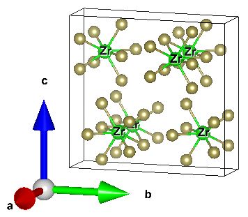
identify potential dark matter sensor materials discussed in Ref. [23] and reveal that one of the
three materials mentioned in the study, the quasi 2-dimensional organic molecular crystal BNQ-
TTF, exhibits various Dirac crossings within the Brillouin zone when spin-orbit coupling is taken
into account. These nodes can potentially be gaped by applying stress and as a result breaking
some of the crystalline symmetries protecting the Dirac nodes.
    In addition to the scattering of sub-MeV DM particles, we also discuss the absorption of bosonic
relics with sub-eV masses. We point out that – in contrast to previous claims – the modulation of
the signal is absent in this case.
    This work is structured as follows. In Sec. 2 we present the general formalism for the calcula-
tion of the expected event rate and its daily modulation, both for the case of DM scattering and
absorption. Sec. 3 provides an improved calculation of the polarization tensor for anisotropic Dirac
materials. Our numerical calculations of the properties of several candidate Dirac materials are
discussed in Sec. 4. In Sec. 5 we then introduce the statistical method that we employ and present
our sensitivity estimates. Finally, we summarize our findings in Sec. 6.

2     Dark Matter Interactions in Dirac Materials
While Dirac materials can in principle be used to probe many different models of sub-MeV DM,
they are particularly well suited for probing U (1) gauge extensions of the Standard Model. These
extensions contain a dark photon A0 which kinetically mixes with the ordinary photon via L ⊃
− 2ε Fµν F 0µν , where Fµν (Fµν
                             0 ) denotes the field strength of the (dark) photon. The dark photon can

either be a DM candidate itself or it can mediate the interactions between another DM particle and
visible matter. The formalism to calculate the resulting detector signals for Dirac materials has
been developed in [21, 22]. For the case of anisotropic Dirac materials, however, we find a number
of pertinent differences with the expressions provided in these works. We will therefore revisit
the derivation of the event rates for DM scattering and absorption in detail and provide improved
formulas.

2.1   Scattering Rates in Dirac Materials
We first consider a DM particle χ with mass mχ which is charged under the new U (1) gauge group.
The total DM-electron scattering rate in a Dirac material with volume V is given by
                                                 Z 3 3 0
                                                   d kd k
                               Rtot = g V Vuc ne           Rk→k0 ,                          (2.1)
                                                    (2π)6

where ne stands for the number of valence band electrons per unit mass and Vuc for the volume of
the unit cell. The factor g = gs gC is the product of spin degeneracy gs and Dirac cone degeneracy
gC [29, 30]. The rate for lifting one electron with initial and final lattice momentum k and k0 from
the valence band into the conduction band reads [31]

                          ρχ σ̄e                                                 g̃(vmin , ψ)
                                     Z
                Rk→k0 =            2
                                        d3 q |FDM (q)|2 |Fmed (q)|2 |fk→k0 (q)|2              , (2.2)
                          mχ 8πµχe                                                   |q|

with the four-momentum transfer q µ = (ω, q) and q = k0 − k. The DM density is denoted by ρχ
and the reduced mass of the DM-electron system by µχe . Furthermore, the fiducial DM-electron

                                                 3
cross section is defined as
µ2χe
σ̄e = |M0 (q0 )|2 . (2.3)
16πm2χ m2e
It is convenient to evaluate the matrix element M0 for scattering on a free electron at q02 = α2 m2e ,
where α and me stand for the fine structure constant and the electron mass respectively. The
momentum-dependence of the scattering, which results from the propagator of the exchanged dark
photon, is then pulled into the form factor [5]
M0 (q) q 2 − m2A0
FDM (q) = = 02 . (2.4)
M0 (q0 ) q − m2A0
In the main part of this work, we will focus on the case of a very light dark photon and, therefore,
neglect mA0 in this expression. The case of a heavy dark photon mediator will be covered in App. A.
Next, we turn to the form factor Fmed (q) which accounts for the optical response of the medium.
More specifically, it parametrizes the ratio of the in-medium scattering amplitude M over the free
amplitude
M(q) jµ0 Dµν jν D00
Fmed (q) = = 0 µν ' , (2.5)
M0 (q) jµ D0 jν D0 00
where j 0 and j denote the DM and the electron current respectively. The difference compared
to the vacuum case manifests in the appearance of the in-medium photon propagator D instead
of the free propagator D0 . In the last step, we used the fact that the scattering process is non-
relativistic, which implies j 0
|j|.1 The in-medium photon propagator can be derived from the
Schwinger-Dyson equation for the electromagnetic field [33, 34]
D−1 = D0−1 − iΠ , (2.6)
where Π stands for the photon polarization tensor. We will explicitly calculate Π for Dirac materials
in Sec. 3. As we will prove there, the spatial components of Π are negligible in the kinematic regime
|q|
ω relevant for DM scattering. Therefore, we obtain
−i q2
D00 (q) ' =⇒ F med (q) = . (2.7)
q 2 − Π00 (q) q 2 − Π00 (q)
The scattering rate, furthermore, depends on the transition form factor fk→k0 , which results from
the electron wave functions in the Dirac material [21, 31],
!
(2π)3 k̃k̃0 + ∆2
2
|fk→k0 (q)| = 1− p p δ(q − (k − k0 )) , (2.8)
2V k̃2 + ∆2 k̃0 2 + ∆2
where 2∆ is the energy gap between the valence band and the conduction band. The tilde indicates
that each three-momentum component is rescaled with the Fermi velocity in the corresponding
direction, for example k̃ = (kx vF,x , ky vF,y , kz vF,z ).
The last ingredient in eq. (2.2) is the velocity integral, which arises from an integration over the
DM velocity distribution f (v):
Z
g̃ = 2|q| f (v) δ (Ef − Ei ) d3 v , (2.9)
1
See derivation of the Coulomb potential in standard text books (e.g. [32])
4where the factor 2|q| has been introduced for convenience. The total energy of the initial and final
state are denoted by Ei and Ef . In the so-called Standard Halo Model, the DM velocity distribution
is given by
(v − ve )2
f (v) = N exp − Θ (vesc − |v − ve |) , (2.10)
v02
where N is a normalization factor, ve is the Earth’s velocity, v0 and vesc are the velocity dispersion
and the Galactic escape velocity and Θ denotes the Heaviside step function. Note that the velocity
distribution only depends on v = |v| and cos θe = v̂ · v̂e (the hat indicates unit vectors), i.e.
f (v) = f (v, cos θe ).
In the non-relativistic limit, the initial and final energy are given by
1
Ei = mχ + me + mχ v 2 − Ek , (2.11)
2
(mχ v − q)2
Ef = mχ + me + + Ek+q . (2.12)
2 mχ
with q again denoting the momentum transfer and
q
Ek = k̃2 + ∆2 . (2.13)
We then find
q2
Ef − Ei = Ek+q + Ek + − q · v ≡ |q| (vmin − v cos θq ) , (2.14)
2 mχ
where we have introduced cos θq = v̂ · q̂ and the minimal velocity
Ek+q + Ek |q|
vmin = + . (2.15)
|q| 2 mχ
The velocity integral can hence be written as
Z 3
d v v
min
g̃ = 2 f (v, cos θe )δ − cos θq . (2.16)
v v
Without loss of generality, we can choose the coordinate system such that the z-axis is aligned
with q. Furthermore, we require the earth velocity vector to reside in the y-z-plane. In spherical
coordinates (v, θ, φ) one then finds θq = θ and
cos θe = sin θ sin φ sin ψ + cos θ cos ψ , (2.17)
where ψ denotes the angle between q and ve . The integration over cos θ then yields 0 if v < vmin
and otherwise sets cos θ = vmin /v. We therefore find
vmin
Z q
v2
g̃ = g̃(vmin , ψ) = 2 vf v, sin φ sin ψ 1 − vmin
2 + cos ψ dvdφ . (2.18)
v>vmin v
An important feature of this result is that it does not depend on |q|. Indeed g̃ is entirely determined
by the two variables vmin and ψ. Calculating this integral numerically and tabulating the results as
a function of two variables is straight-forward. The result is shown in Fig. 1 and confirms the naive
expectation that scattering in the direction of the DM wind (i.e. ψ ≈ 0) is strongly preferred.
5π π
˜
log10 g(vmin ,ψ)
3 3
4
π 4
π
3
2
1
1 1
π π
ψ
2 2 0
-1
-2
1 1 -3
π π
4 4
-4
-5
0 0
0 100 200 300 400 500 600 700
vmin [km/s]
Figure 1: The anisotropic velocity integral g̃(vmin , ψ).
We can now transform into the laboratory frame, in which ve is time-dependent. We adopt the
same coordinate system as proposed in Ref. [18], in which ve points in the z-direction at t = 0 days
and lies in the y-z-plane at t = 0.5 days:
sin αe sin β
ve (t) = ve sin αe cos αe (cos β − 1) , (2.19)
cos αe2 + sin αe2 cos β
where αe = 42◦ is the angle between the Earth’s rotation axis and its velocity and β = 2π ×t/1days.
Finally, ψ is obtained from cos ψ = v̂e · q̂.
In order to understand the impact of the Earth’s rotation on the DM scattering rate, it is
instructive to consider collisions with ψ = 0 which dominate the velocity integral. For those, we
can derive the inequality s
2 +4 ∆ ,
vmin ≥ vF,i (2.20)
mχ
with approximately i = z (i = y) at t = 0 (t = 0.5). The fraction of DM particles which can
undergo scattering, hence, strongly depends on the Fermi velocity in the direction of the DM wind.
This implies strong daily modulations of the scattering rate in anisotropic Dirac materials with
vF,y 6= vF,z .
A final subtlety arises from the fact that the analogy between the electron and a free Dirac
fermion only applies for sufficiently small momenta k. For larger momenta, the dispersion relation
of the electron will deviate from eq. 1.1. Of course, electrons with such large momenta may still
contribute to the event rate, but the formalism outlined above cannot be applied. To obtain a con-
servative estimate of the event rate, Ref. [21] introduced a cut-off Λ and considered only scattering
processes for which k, k0 < Λ. For a known band structure the cut-off Λ can be determined by
identifying the momentum for which the dispersion relation becomes non-linear.
In the case of an anisotropic Dirac material the definition of Λ becomes more subtle. Indeed,
in this case the cut-off momentum typically depends on the direction, Λ = (Λx , Λy , Λz ). While in
principle it would be possible to apply different cut-offs in different directions, we will again adopt
6a simpler and more conservative approach and require
k̃, k̃ 0 < min(Λx vF,x , Λy vF,y , Λz vF,z ) ≡ Λ̃ . (2.21)
Note that this prescription differs from the one proposed in Ref. [21], where the maximum is taken
rather than the minimum (presumably because of a typographical mistake).
2.2 Absorption of Dark Photon Dark Matter
Let us now consider the case that the dark photon itself constitutes the DM. It can then be absorbed
in a Dirac material in analogy to the photoelectric effect. Specifically, we are interested in the
absorption of non-relativistic dark photons with rest mass comparable to the band gap, which
implies that ω ' mA0
|q|. In this regime – as we will show in the next section – the spatial
components of the in-medium photon propagator can be approximated as
−ig ij
Dij = . (2.22)
q 2 + Πii (q)
We now want to determine the effective in-medium mixing angle εmed between the dark and
the ordinary photon. For anisotropic materials εmed depends on the polarization. Since the dark
photons are non-relativistic, we can conveniently choose the polarization vectors
(x )µ = (0, 1, 0, 0) , (y )µ = (0, 0, 1, 0) , (z )µ = (0, 0, 0, 1) . (2.23)
The in-medium mixing angle for an x-polarized dark photon is then obtained from the relation2
εmed,x (x )µ ≡ ε m2A0 Dµν (x )ν , (2.24)
which implies
m4A0
|εmed,x |2 = ε2 2 . (2.25)
m2A0 + Π11 (mA0 )
In the above expression we explicitly indicate that the polarization tensor has to be evaluated at
q 2 = m2A0 . The x-polarized dark photon absorption rate is determined from the optical theorem
(see e.g. [36])
|εmed,x |2 (x )µ Im Πµν (x )ν |εmed,x |2 Im Π11
Γx = = . (2.26)
ω m A0
Absorption rates for the other two polarizations are obtained in complete analogy. One simply has
to replace Π11 by Π22 (Π33 ) for y-polarized (z-polarized) dark photons.
In principle the incoming dark photon polarization needs to be evaluated in the laboratory frame.
This complication is, however, usually irrelevant since the dark photons in the solar neighborhood
are expected to be unpolarized. Therefore, the rate is simply given by the average
1 |εmed,x |2 Im Π11 + |εmed,y |2 Im Π22 + |εmed,z |2 Im Π33
Γ= (Γx + Γy + Γz ) = . (2.27)
3 3 mA0
The total absorption rate in the detector per unit mass is obtained as
ρA0
Rtot = Γ. (2.28)
ρT mA0
2
The analogous expression for longitudinal, transverse polarization can e.g. be found in [35].
7The lowest dark photon mass which can be probed by a Dirac material is set by the band gap.
Furthermore, the rate has to be cut off when the largest energy deposit consistent with the linear
dispersion relation is reached at mA0 = 2Λ̃ [21].
We emphasize that the absorption of unpolarized dark photons is time-independent. This is
because the spatial components of the polarization tensor Πii (with i = 1, 2, 3) are independent
of the three-momentum transfer (in the relevant limit ω
|q|). This statement disagrees with
Ref. [22] which found a large daily modulation in anisotropic Dirac materials. The discrepancy
arises because the photon polarization tensor employed in Ref. [22] carries a residual q̃2 -dependence
which would favor scattering in the direction of the largest Fermi velocity. We will show in the next
section that such a momentum dependence is absent and that the absorption rate remains constant
with time.
3 Polarization Tensor in Dirac Materials
In this section, we will derive the photon polarization tensor for Dirac materials. The Lagrangian
describing photons and electronic excitations in Dirac materials reads
1
L = − Fµν F µν + i ψ̄γ̃ µ (∂µ + ieAµ )ψ − ∆ψ̄ψ . (3.1)
4
For convenience, we introduced the rescaled gamma matrices
γ̃ µ = {γ0 , vF,x γ1 , vF,y γ2 , vF,z γ3 } . (3.2)
Compared to the Lagrangian of quantum electrodynamics, the speed of light is replaced by the
Fermi velocity in the corresponding spatial direction. Furthermore, the role of the electron mass
term is played by ∆ which is half the band gap. Notice that the structures of the electron kinetic
term and the electron-photon vertex coincide as required by gauge invariance.
q
Figure 2: Feynman diagram for the polarization tensor
At first order in perturbation theory, the photon polarization tensor is obtained from the diagram
shown in Fig. 2. The corresponding amplitude reads
( )
(−ie)2g Z d4k i i
Πµν (q) = − Tr γ̃ µ γ̃ν , (3.3)
κ 2 (2π)4 k˜ − ∆
k˜ + ˜q − ∆
where the rescaled four-momenta q̃ µ and k̃ µ are defined analogous to γ̃ µ in eq. (3.2). The case of a
single Dirac fermion in the loop corresponds to a single Dirac cone (gC = 1) with spin-degeneracy
gs = 2. We keep the factor g in the above expression in order to allow for generic Dirac cone
degeneracy. The background dielectric constant κ is taken to be isotropic for the moment (the
8case of anisotropic κ will be discussed below). In order to employ the well-known result for the
vacuum polarization tensor in QED (see e.g. Ref. [32]), it is convenient to transform the integration
measure from k to k̃. Furthermore, we need to regularize the integral. Choosing the dimensional
regularization scheme, we perform the following replacement
d4 k → (vF,x vF,y vF,z )−1 µ̃4−d dd k̃ , (3.4)
where µ̃ denotes the renormalization scale. The resulting polarization tensor can be written in the
form 2 2
−qx vF,x − qy2 vF,y
2 − q2v2 2 2 2
z F,z ωqx vF,x ωqy vF,y ωqz vF,z
−ωqx vF,x2 ω 2 vF,x
2 0 0 π(q̃ 2 )
Πµν (q) = , (3.5)
2
−ωqy vF,y 0 2 2
ω vF,y 0 κ
2
−ωqz vF,z 0 0 ω 2 vF,z
2
where we neglected quartic terms in the vF,i . This is justified since the Fermi-velocities are much
smaller than the speed of light. For later convenience, we have not included κ in the definition of
π(q̃ 2 ). As a consistency check, one can easily verify that the polarization tensor fulfills the Ward
identities Πµν qµ = Πµν q ν = 0. This implies that the photon remains massless within the Dirac
material. Let us now turn to the polarization function. We find
Z1 2−d/2
4g e2 µ̃2
2 d
π(q̃ ) = − dx x (1 − x) Γ 2 − 2 (3.6)
(4π)d/2 vF,x vF,y vF,z ∆2 − x(1 − x)q̃ 2
0
In the modified minimal subtraction scheme (MS), one replaces
Γ 2 − d2 2−d/2
1
A −→ log A , (3.7)
(4π)d/2 (4π)2
and hence
Z1
g e2 µ̃2
2
π(q̃ ) = − 2 dx x (1 − x) log . (3.8)
4π vF,x vF,y vF,z ∆2 − x(1 − x)q̃ 2
0
In the following, we set the renormalization scale to the cutoff Λ̃. This choice is motivated by
√
the matching condition for the effective electron charge which is given by e/ κ at the cutoff (where
electrons should behave as in an insulator). In order to recover the standard expression of Π00 for
an isotropic Dirac material with vanishing band gap (see e.g. [37]), the precise replacement is
µ̃ → 2 e−5/6 Λ̃ (3.9)
The imaginary part of the polarization function, which arises from a negative argument in the
logarithm, can be evaluated analytically. One finds
1
ge 2 4 e−5/3 Λ̃2
Z
π(q̃ 2 ) = − 2 dx x (1 − x) log
4π vF,x vF,y vF,z ∆2 − x(1 − x)q̃ 2
0
2
s 2
iπ 2∆ 4∆
1 − 2 Θ q̃ 2 − 4∆2 .
+ 1+ 2 (3.10)
6 q̃ q̃
9For convenience we also state the result for vanishing band gap,
!
2 g e2 4Λ̃2
log 2 + iπΘ q̃ 2
π(q̃ ) = − . (3.11)
24π 2 vF,x vF,y vF,z q̃
We finally want to generalize the photon polarization tensor to the case of an anisotropic background
dielectric tensor. Along the principal axes, the latter can be chosen diagonal such that we have
κxx 0 0
κ = 0 κyy 0 . (3.12)
0 0 κzz
Given this form, the spatial components of the polarization tensor can be obtained by the replace-
ment Πii /κ → Πii /κii in eq. (3.5) [21]. The remaining components are fixed by the Ward identities.
The most general expression for the polarization tensor thus reads
2
vF,z 2
vF,y 2
vF,z 2
vF,x 2
vF,y 2
vF,z
−q 2 2 2
− qy κyy − qz κzz ωqx κxx ωqy κyy ωqz κzz
x κxx 2 2
vF,x 2 vF,x
−ωqx κxx ω κxx 0 0
µ π(q̃ 2 ) .
Π ν (q) = 2
vF,y 2
vF,y
(3.13)
2
−ωq y κyy 0 ω κyy 0
v2 v2
−ωqz κF,z
zz
0 0 ω 2 κF,z
zz
Notice that in the kinematic regime relevant for DM scattering |q|
ω, the polarization tensor is
strongly dominated by the Π00 -component. With this simplification, the Schwinger-Dyson equation
leads to the photon propagator of eq. (2.7) and therefore
1
Fmed (q) = 2 2 2
. (3.14)
vF,z vF,y vF,z π(q̃ 2 )
2 2 2
1 + qx κxx + qy κyy + qz κzz q2
This expression improves the corresponding expression in Ref. [21], where the geometric mean of
the components of κ is taken instead of including them individually.
In the opposite regime ω
|q| which is relevant for dark photon absorption, the spatial compo-
nents of Π dominate and one obtains the photon propagator of eq. (2.22). We make the important
observation that for ω
|q|, Πij becomes independent of the three-momentum q (since the func-
tion π(q̃ 2 ) in (3.13) only depends on ω 2 in this regime). As stated earlier, this implies that the
dark photon absorption rate in Dirac materials does not depend on the direction of the momentum
transfer.
4 Candidate Dirac Materials
For our study we consider three potential candidates for Dirac materials based DM sensors: ZrTe5 ,
Yb3 PbO, and BNQ-TTF. In this section we present calculations of their respective band structures
and determine the relevant properties. The ab initio calculations were performed in the framework of
the density functional theory (DFT) using a pseudopotential projector augmented-wave method [38–
41], as implemented in the Vienna Ab initio Simulation Package (VASP) [42, 43]. We compare
10results for the experimental crystal structure (NR) with results from structurally optimized crystal
structures, which where obtained by allowing the unit cell volume to change, but keeping the unit
cell shape and the atomic positions unchanged (ISIF7). For the structural optimization and the
band structure calculations, we have used the semilocal meta-GGA functional (SCAN) [44, 45]. To
get reliable optimized structural ground states we added Van der Waals corrections according to
Tkatchenko and Scheffler [46] for the calculations concerning ZrTe5 and BNQ-TTF.
For the ~k-space integration, we chose a Γ-centered mesh [50] with 14×4×4 points for ZrTe5 ,
10 × 10 × 10 points for Yb3 PbO, and 14×8×2 points for BNQ-TTF. The cut-off energy was set
to 600 eV. The calculation of the dielectric tensor was performed using the generalized gradient
approximation according to Perdew, Burke, and Ernzerhof [51] and density functional perturbation
theory. The calculations for the band structure and dielectric tensor were performed with spin-
orbit coupling, the structural optimization was done without spin-orbit coupling. For Yb3 PbO the
f -electrons are considered to be occupied. To push related electronic bands occurring at the Fermi
level into the valence band we applied the GGA+Hubbard-U correction using a value of U = 10 eV
for the Yb-f -orbitals as suggested in Ref. [28].
The unit cells and obtained lattice parameters from the structural optimization in comparison
with the reported experimental lattice constants are shown in Fig. 3. We observe that the overall
unit cell volume for the computational ground state is slightly decreased for ZrTe5 and Yb3 PbO
and slightly increased for BNQ-TTF. The increase of the unit cell volume for the structural ground
state for organic materials is common and can be traced back to a slightly increased bond length
(a) (b) (c)
Material Space Group a b c α β γ VUC ρ ne
(Å) (Å) (Å) (Å3 ) (gcm−3 ) (1023 kg−1 )
ZrTe5 Cmcm (63) Exp. [47] 3.987 14.53 13.722 90 90 90 795.146 6.089 2.065
this work 3.978 14.494 13.690 90 90 90 789.292 6.135 2.065
Yb3 PbO Pm3m (221) Exp. [48] 4.859 4.859 4.859 90 90 90 114.700 10.744 8.115
this work 4.737 4.737 4.737 90 90 90 106.272 11.596 8.115
BNQ-TTF P21 /n (14) Exp. [49] 3.881 7.532 31.350 90 96.476 90 916.365 1.683 6.480
this work 3.899 7.567 31.698 90 96.476 90 929.339 1.659 6.480
(d)
Figure 3: Crystal structure information of the considered Dirac materials. (a)-(c) show the unit cells
ZrTe5 , Yb3 PbO, and BNQ-TTF. (d) Experimental and computational lattice constants, unit cell
volumes, and densities. The electron density ne specifies the density obtained for a single electron
per unit cell.
110.60
0.50 1.00
0.40
Energy (eV)
Energy (eV)
Energy (eV)
0.20
0.00 0.00
0.00
−0.20
−0.50 −1.00
−0.40
Y ΓZ T SΓ X R Γ X M Y Γ YΓZ C D Z E Γ BA Γ
Figure 4: Calculated ab initio band structures for potential Dirac DM sensor materials: ZrTe5 (left),
Yb3 PbO (center), and BNQ-TTF (right).
Material Mode vF,x vF,y vF,z ∆ Λx Λy Λz ~kcone
(c) (c) (c) (meV) (Å−1 ) (Å−1 ) (Å−1 )
ZrTe5 NR 1.1×10⁻³ 4.5×10⁻⁴ 1.0×10⁻³ 11.8 0.23 0.215 0.1 (0.,0.,0.)
ISIF7 1.1 × 10⁻³ 4.4 × 10⁻⁴ 9.1 × 10⁻⁴ 15.6 0.23 0.216 0.1 (0.,0.,0.)
Th. [21] 2.9×10⁻³ 5.0×10⁻⁴ 2.1×10⁻³ 17.5 0.07 0.07 0.07 (0.,0.,0.)
Exp. [52] 1.3×10⁻³ 6.5×10⁻⁴ 1.6×10⁻³ 11.75 (0.,0.,0.)
Yb3 PbO NR 8.5×10⁻⁴ 8.8×10⁻⁴ 8.8×10⁻⁴ 17.2 0.45 0.45 0.45 (±0.185,0.,0.0)
8.8×10⁻⁴ 8.5×10⁻⁴ 8.8×10⁻⁴ (0.0,±0.185,0.0)
8.8×10⁻⁴ 8.8×10⁻⁴ 8.5×10⁻⁴ (0.0,0.0,±0.185)
ISIF7 8.7×10⁻⁴ 9.0 × 10⁻⁴ 9.0 × 10⁻⁴ 19.4 0.45 0.45 0.45 (±0.185,0.,0.0)
9.0 × 10⁻⁴ 8.7×10⁻⁴ 9.0 × 10⁻⁴ (0.0,±0.185,0.0)
9.0 × 10⁻⁴ 9.0 × 10⁻⁴ 8.7×10⁻⁴ (0.0,0.0,±0.185)
Impl. 8.9 × 10⁻⁴ 8.9 × 10⁻⁴ 8.9 × 10⁻⁴ 19.4 0.45 0.45 0.45
BNQ-TTF NR 2.3 ×10⁻⁴ 1.9 ×10⁻⁴ - 0. 0.81 0.3 0.1 (±0.075,0.,0.5)
1.9 ×10⁻⁴ 2.3 ×10⁻⁴ - 0.3 0.81 0.1 (±0.075,0.,0.)
ISIF7 2.2 ×10⁻⁴ 1.8 ×10⁻⁴ - 0. 0.81 0.3 0.1 (±0.065,0.,0.5)
1.8 ×10⁻⁴ 2.2 ×10⁻⁴ - 0.3 0.81 0.1 (±0.065,0.,0.)
Impl. 2.0 × 10⁻⁴ 2.0 × 10⁻⁴ 1.0 × 10⁻⁴ 5.0 0.3 0.3 0.1
Table 1: Calculated Fermi-velocities, band gaps, cut-off radii, and Dirac point positions in the
Brillouin zone. We compare values obtained using optimized structures (ISIF7) and experimental
structures (NR). The values implemented for our sensitivity estimates are highlighted in bold.
occurring in the DFT calculations.
The obtained band structures for ZrTe5 , Yb3 PbO, and BNQ-TTF are shown in Fig. 4. ZrTe5
exhibits a gaped Dirac point at Γ, the center of the Brillouin zone. The calculated band gap with
and without structural optimization are given by 31.2 meV and 23.6 meV, which corresponds to
∆ = 15.6 meV and ∆ = 11.8 meV, respectively. Yb3 PbO exhibits a gaped Dirac point along the
path ΓX (Γ = (0, 0, 0), X = (0.5, 0, 0)) located at ~kD = (0.185, 0.0, 0.0). The corresponding band
gap is 34.4 meV (∆ = 17.2 meV) for the experimental unit cell and 38.8 meV (∆ = 19.4 meV)
for the optimized unit cell. Due to the cubic symmetry of the system a total of 6 such points can
be observed which can be projected by applying 4-fold rotations about the ky - and kz - axis in the
Brillouin zone.
In Ref. [23], BNQ-TTF was discussed as a tiny gap organic semiconductor. However, our
calculations incorporating spin-orbit coupling reveal a Dirac crossing along the paths DZ (D =
(0.5, 0.0, 0.5), Z = (0.0, 0.0, 0.5)) and ΓB (B = (0.5, 0.0, 0.0)) at kx = 0.075 for the experimental
and kx = 0.065 for the optimized unit cell. By two-fold rotational symmetry both points come
12Material Mode κxx κyy κzz κxy κxz κyz κyx κzx κzy g
ZrTe5 This work 308.4 20.75 126.1 -0.97 -1.2 -0.38 0.5 -1.2 -0.02 2
ZrTe5 Ref. [21] 187.5 9.8 90.9
Yb3 PbO This work 42.8 42.8 42.8 -12.38 8.58 -12.38 8.58 -12.38 8.58 12
BNQ-TTF This work 18.7 5.6 10.3 -0.05 0.07 -1. -0.05 0.07 -1. 8
Table 2: Dielectric tensor for ZrTe5 , Yb3 PbO, and BNQ-TTF calculated using density functional
perturbation theory. In the final column we also specify the respective degeneracy g = gs gC .
with a partner with the corresponding values at −kx . Organic materials are soft and therefore this
material can be tuned by applying stress. A slightly strained sample of BNQ-TTF breaking the
space group symmetries of the material is therefore likely to introduce a tiny gap. For our sensitivity
estimates in the following section, we will consider a band gap of 10 meV (∆ = 5 meV).
We furthermore performed additional band structure calculations for all three materials to fit
the occurring Fermi velocities and determine the cut-off radii Λi where the Dirac dispersion approxi-
mately holds. All values are summarized in Tab. 1. The highest Fermi velocities are found for ZrTe5
which are of the order of 10−3 . In contrast, the flat bands of BNQ-TTF lead to very small Fermi
velocities in the order of 10−4 . Due to the low symmetry of ZrTe5 and BNQ-TTF all three Fermi
velocities come with different values. Furthermore, BNQ-TTF is a quasi 2-dimensional material
were the dispersion in the kz direction of the Brillouin zone is extremely flat and the corresponding
Fermi velocity vanishes. This effect is related to the weak hopping of electrons in the c-direction of
the crystal stemming from the layered structure of the material. Applying pressure on the sample
along the crystallographic c-direction will decrease the distance of molecules in the c-direction and
therefore increase the hoping amplitudes between the molecules. As a result, an increased hopping
amplitude will lead to a stronger dispersion of bands opening the opportunity to lift the flatness of
the band and tune the Fermi velocity. In the following, we assume that in a sufficiently strained
sample the flat direction will take a value of vF,z = 10−4 for our sensitivity estimates.3
In comparison to ZrTe5 and BNQ-TTF, Yb3 PbO crystallizes in a high-symmetry space group
Pm3m. As the Dirac point is observed, e.g., along the path ΓX the little group of ~k is given by
C4v [54, 55]. Hence, the rotational symmetry enforces the two Fermi velocities corresponding to the
directions orthogonal to ΓX to be degenerated, i.e., vF,y = vF,z 6= vF,x . For Yb3 PbO we observe
slightly different values for vF,i in the conduction and the valence bands. In the conduction (valence)
band, the value for vF,x is about vF,x ≈ 2vF,y (vF,x ≈ 21 vF,y ). Hence the averaged values for vF,x
given in Tab. 1 do not reflect this anisotropy. In the following we will use these averaged values
to estimate the sensitivity of Yb3 PbO, but we will not attempt to calculate the modulation signal,
which would require an extended formalism allowing for different Fermi velocities in the valence and
conduction band.
We furthermore calculated the values for the dielectric tensor by using density functional per-
turbation theory as implemented in the code VASP. The values are given in Tab. 2. Due to the
tiny gaps present in these materials these calculations are very sensitive to the gap size. However,
we observe that for all three materials the diagonal elements κxx , κyy , and κzz dominate over the
3
We note that for small Fermi velocities the effective coupling strength αeff = α/(κ vF ) increases and the material
becomes increasingly strongly coupled. The considered Fermi velocities of BNQ-TTF imply αeff ∼ 10. It is conceivable
that perturbation theory still applies to systems with αeff in this range (see discussion in [30]). Indeed, this has
experimentally been verified for the case of graphene [53]. Nevertheless, we wish to point out that our one-loop
calculation of the polarization tensor should only be seen as qualitative estimate for the case of BNQ-TTF.
13off-diagonal components. The largest values are found for ZrTe5 which is highly anisotropic with
κxx ≈ 308, but κyy ≈ 21. The smallest values are seen for BNQ-TTF with κxx ≈ 19 and κyy ≈ 6.
The cubic symmetry in Yb3 PbO enforces κxx = κyy = κzz ≈ 43.
Finally, we need to determine the optimum orientation of the three Dirac materials in the
laboratory. The coordinate system that we introduced above implies that the DM wind points in
the z-direction at t = 0 days and approximately in the y-direction at t = 0.5 days. We hence want
to align the materials in such a way that the largest anisotropy is observed in the y-z plane. In the
following, we will always align the materials such that the smallest Fermi velocity points in the y
direction, while the largest Fermi velocity points in the z direction.4 Since the event rate is largest
when the DM wind is aligned with the smallest Fermi velocity, we expect a daily modulation that
peaks at t = 0.5 days.
5 Sensitivity Estimates
We are now in the position to calculate the predicted DM signal as a function of time in the Dirac
materials that we consider and to estimate their sensitivity. Before presenting our results, we first
introduce the statistical approach that we employ.
5.1 Statistical Method for Daily Modulation
We will consider two possible outcomes for the experiments under consideration. First, we consider
the case that the DM hypothesis is incorrect and that the experiments do not observe any DM signal.
For example, if no events are observed at all, any parameter point predicting 3 or more events can be
excluded at 95% confidence level. If the experiment observes a number Nb of background events, it
can still exclude all parameter points for which the probability to observe at most Nb signal events
is less than 5%.5
The second outcome we consider is that the experiments do observe a DM signal. In this case it
will be essential to confirm the DM nature of the excess by performing a test for daily modulation.
Whether or not the daily modulation will be observable depends on both the amplitude of the
modulation and the total (i.e. unmodulated) rate. We use the following approach to quantify the
significance of the daily modulation.
Each day of observation is divided into the twelve hours around the expected maximum of
the modulation and the twelve hours around the minimum of the modulation. Let Nmax be the
total number of events that fall into the former window and Nmin the remaining events. Assuming
Nmax , Nmin
1 the√event numbers √ are expected to follow a normal distribution with estimated
standard deviation Nmax and Nmin respectively. Hence, √ the difference Nmax − Nmin should
follow a normal distribution with standard deviation Nmax + Nmin . In the absence of a daily
modulation, the expectation value of this quantity vanishes. To test the hypothesis that there is no
modulation, we can hence define the test statistic
(Nmax − Nmin )2
χ2s = , (5.1)
Nmax + Nmin
4
For BNQ-TTF the two larger Fermi velocities are nearly degenerate. We align the detector such that the dielectric
constant is smallest in the z direction.
5
A stronger bound can be obtained if a background model exists that would allow for background subtraction.
Here we focus on the most conservative case in which no background model is assumed.
14which we have confirmed to follow a χ2 distribution with one degree of freedom under the null
hypothesis using explicit Monte Carlo simulation. If χ2s
1 there is positive evidence for a daily
modulation and the hypothesis of no modulation can be rejected. For example, to reject the null
hypothesis at 95% confidence p level, one would require χ2s > 3.84. More generally, the significance
of the modulation is given by χ2s standard deviations.
In the following it will be useful to define the total number of signal events Ns = Nmax + Nmin
and the modulation fraction A = (Nmax − Nmin )/(Nmax + Nmin ). With this definition, the test
statistic can simply be written as χ2s = A2 Ns . Hence, for a modulation fraction of A = 20% it is
necessary to observe Ns ≈ 225 events to detect 3σ evidence for a modulation, while for A = 50%
fewer than 40 events may be sufficient. Note that given actual data, more sophisticated methods,
such as a Lomb-Scargle [56, 57] analysis, may reveal even higher significance for a modulation (see
e.g. [58]).
Our approach is easily extended to include a number Nb of background events. Assuming that
the background does not modulate, it will cancel in the numerator but contribute to the denominator
of eq. (5.1), giving
(Nmax − Nmin )2 Ns
χ2sb = = χ2s . (5.2)
Nmax + Nmin + Nb Ns + Nb
We emphasize that this expression corresponds to the most conservative case without background
subtraction and does not require any model of the expected background.
Let us consider the example of an unknown background which has a rate of 1 event per day. The
total exposure is assumed to be 1 kg year. Based on the total number of observed events alone one
can exclude all parameter points that would predict more than ∼400 signal events. Nevertheless,
provided the modulation amplitude is sufficiently large, a substantially smaller number of signal
events may be sufficient to identify a daily modulation. Indeed, given a modulation fraction of
50% (30%) it would only require about 135 (250) signal events to obtain 3σ evidence for daily
modulation.
5.2 Results for Dark Matter Scattering
We present our main results in Fig. 5 for three different Dirac materials. The two panels in the
top row show the expected sensitivity for ZrTe5 , assuming the Fermi velocities and the band gap
obtained from our calculations (left) and from experimental measurements (right). The two panels
in the bottom row correspond to BNQ-TTF and Yb3 PbO, respectively. In each panel the dashed
line indicates the exclusion bound from a null result, the shaded region in the first three panels
indicates the parameter space where a daily modulation can be identified with 3σ significance. For
the moment we assume that experimental backgrounds are negligible.
For comparison we show in each panel the combination of parameters for which the observed
DM relic abundance can be reproduced via the freeze-in mechanism in a model with a massless
dark photon. We include the contribution from plasmon decays, recently studied in Refs. [9, 10, 59].
In the top row we furthermore indicate two benchmark points, corresponding to mχ = 20 keV,
σe = 2 · 10−41 (orange) and mχ = 50 keV, σe = 3 · 10−41 . The predicted event rate for these two
points as a function of time is shown in Fig. 6.
We make the surprising observation that the modulation signal is extremely sensitive to the
assumed properties of the Dirac material. For the case of ZrTe5 both the total rate and the mod-
ulation amplitude differ substantially for the different values of the Fermi velocities and the band
gap. This is investigated more closely in Fig. 7, which in the left panel shows the derivative of
1510-36 10-36
3σ evidence for 3σ evidence for
10-37 daily modulation 10-37 daily modulation
10-38 t 10-38 t
rge rge
n ta n ta
-39
ez e -i -39 e -i
10
Fre
10
Fr eez
10-40 10-40
⨯ ⨯
σe [cm2 ]
σe [cm2 ]
⨯ ⨯ nts
Cooling constraints
Cooling constraints
10-41 10-41
d eve
10-42 s 10-42 ecte
vent exp
ed e 3
pect
10-43 3 ex 10-43
10-44 10-44
ZrTe 5 (th., 1 kg year) ZrTe 5 (exp., 1 kg year)
10-45 No background 10-45
No background
10-46 10-46
10 100 1000 10 100 1000
mχ [keV] mχ [keV]
10-36 10-36
3σ evidence for
10-37 daily modulation 10-37
10-38 t 10-38 t
rge rge
-i n ta n ta
-39
eze -39 e -i
10
Fre
10
Fr eez
-40
10 10-40
σe [cm2 ]
σe [cm2 ]
Cooling constraints
Cooling constraints
10-41 10-41
10 -42
ve nts 10-42 events
ed
e 3 expected
10 -43
xpect 10 -43
3e
10-44 10-44
-45
BNQ-TTF (1 kg year) Yb3 PbO (1 kg year)
10 10-45
No background No background
10-46 10-46
10 100 1000 10 100 1000
mχ [keV] mχ [keV]
Figure 5: Expected sensitivity for the Dirac materials ZrTe5 , BNQ-TTF and Yb3 PbO. The two
panels in the top row correspond to different assumed properties for ZrTe5 (see text for details). In
the case of a null result, all parameter points above the dashed lines (corresponding to 3 expected
events) can be excluded. In the shaded parameter region it will be possible to identify a daily
modulation with 3σ significance in the case that a DM signal is observed.
the total rate with respect to the cosine of the angle ψ between the momentum transfer q and the
velocity of the Earth ve . We can see that for t = 0.5 days (i.e. close to the maximum of the rate)
the differential event rate looks similar in the two cases and is strongly peaked towards cos ψ = 1,
such that the momentum transfer is aligned with the direction of the DM wind.
For t = 0 days on the other hand, there are decisive differences between the two cases. While
for the theoretically calculated Fermi velocities and band gap the differential rate still peaks at
cos ψ = 1, for the experimental values scattering with cos ψ ≈ 1 is strongly suppressed. This can
be traced back to the fact that in this case the Fermi velocity pointing in the direction of the DM
wind is vF = 1.6 · 10−3 and hence close to the maximum velocity of DM particles in the Galactic
halo. As a result, only very few DM particles have sufficient kinetic energy to induce scattering
with cos ψ ≈ 1 and the event rate is suppressed.
161000 mχ = 50 keV, σe = 3 ⨯ 10-41 cm2 1000
mχ = 50 keV, σe = 3 ⨯ 10-41 cm2
Rtot [kg-1 days-1 ]
Rtot [kg-1 days-1 ]
500 500
mχ = 20 keV, σe = 2 ⨯ 10-41 cm2
100 100
mχ = 20 keV
σe = 2 ⨯ 10-41 cm2
50 50
ZrTe 5 (th.) ZrTe 5 (exp.)
0.0 0.2 0.4 0.6 0.8 1.0 0.0 0.2 0.4 0.6 0.8 1.0
t [days] t [days]
Figure 6: Event rate in ZrTe5 as a function of time for the two benchmark points indicated in Fig. 5.
The two panels correspond to different assumptions on the material properties.
As a result, for the theoretically calculated properties of ZrTe5 we find a larger total rate but a
smaller modulation amplitude than for the experimentally measured properties. This is illustrated
in the right panel in Fig. 7, which shows the modulation amplitude (blue) and the significance
for a daily modulation for σe = 10−41 cm2 (orange) in the two cases. We can see that for the
experimentally measured properties the modulation amplitude is substantially larger and hence the
significance of a daily modulation is increased in spite of the smaller total rate.
Finally, we note that for the theoretical properties of ZrTe5 the amplitude of the modulation
vanishes for mχ ∼ 500 keV and becomes negative for larger DM masses. This is a result of two
competing effects: The velocity integral gives the largest contribution if the DM wind points in the
direction of the smallest Fermi velocity. At the same time, the combination of form factors FDM and
fk→k0 favors small q but large q̃. It, hence, prefers scattering in the direction of the larger Fermi
velocities. For small DM masses, the former effect dominates and leads to a modulation peaked at
t = 0.5 days while for larger DM masses the second effect can be comparable or even dominant.6
This can lead to a vanishing modulation amplitude for specific values of the DM mass or even an
anti-modulation peaked at t = 0 days. Since our definition of χ2 is symmetric in Nmax and Nmin
the case of anti-modulation is automatically included in our test for daily modulation.
An interesting side remark concerns the dark matter form factor. Since we focused on the
exchange of a light dark photon mediator, the latter was taken to scale as FDM ∝ q −2 with the
four-momentum transfer. This behavior changes if we consider heavy mediator exchange for which
FDM approaches a constant. We find that the momentum scaling of FDM has profound implications
on the modulation of the DM scattering rate. For illustration, we depict the sensitivity of Dirac
materials for the heavy mediator case in App. A. Most remarkably, the modulation fraction is
increased and the flip in the modulation amplitude at mχ ∼ 500 keV completely disappears for
ZrTe5 .
Thanks to its tiny band gap the organic Dirac material BNQ-TTF can probe significantly smaller
6
This is because the minimal velocity for scattering vmin decreases with mass (cf. 2.20) such that the suppression
of the velocity integral in the direction of the large Fermi velocity becomes less pronounced.
17500 100 102
ZrTe5 (th.)
χ2 (σe = 2 ⨯ 10-41 cm2 )
ZrTe5 (exp.) t = 0.5 days
d R / d cos ψ [kg-1 year-1 ] 3σ evidence
Modulation fraction
100 101
mDM = 20 keV
50
10-1 100
10
t = 0 days
5
10-1
ZrTe5 (th.)
1 ZrTe5 (exp.)
0.5
10-2 10-2
0.0 0.2 0.4 0.6 0.8 1.0 10 100
cos ψ mχ [keV]
Figure 7: Left: Differential event rate with respect to the cosine of the angle ψ between the velocity
of the Earth and the momentum transfer at t = 0 days (blue) and t = 0.5 days (orange) for the
theoretically calculated properties of ZrTe5 (solid) and the experimentally measured properties
(dashed). Right: Modulation amplitude (blue, left y-axis) and significance (orange, right y-axis) of
a daily modulation for the two cases.
DM masses than ZrTe5 . For the assumed value ∆ = 5 keV the sensitivity extends down to mχ >
4 keV. Close to the threshold the modulation amplitude is found to be quite large, but it decreases
rapidly for heavier DM particles and switches sign for mχ > 100 keV.
For the last material Yb3 PbO we only show the sensitivity based on the absolute rate. The
modulation signal is suppressed due to the very symmetric nature of this material.
Finally, we consider the case where backgrounds are non-negligible and assume for concreteness
a background rate of 1 event per kg day (corresponding to 365 events from background in the
assumed exposure of 1 kg year). The estimated sensitivities in this case are shown in Fig. 8. In
this case, only parameter points predicting more than 400 signal events can be excluded based on
the absolute rate, and the resulting bounds are therefore much weaker than in Fig. 5. However, the
parameter region where a DM signal can be identified based on its daily modulation remains almost
unchanged. In fact, for DM masses close to the kinematic threshold, the modulation fraction can
be so large that a DM signal can be identified even if the DM signal is significantly smaller than
the number of background events.
To conclude this discussion, let us briefly comment on the dependence of our results on the
cut-off Λ. It is clear that introducing such a cut-off leads to conservative results for the total rate,
since only a part of the Brillouin zone is included in the calculation. However, for the modulation
amplitude it could in principle happen that the region excluded from the calculation contributes to
the modulation with the opposite phase and would hence reduce rather than increase the modulation
amplitude. We have therefore explicitly confirmed that variations in the cut-off Λ do not significantly
modify any of the results presented in this section. The reason is that the dominant contribution to
DM scattering stems from collisions with small momentum transfer, for which the precise value of
the cut-off is irrelevant. Only if the modulation amplitude nearly vanishes (i.e. close to the transition
from modulation to anti-modulation) can the dependence on Λ be sizeable. Since the search for a
daily modulation is essentially insensitive in this particular region, this dependence on Λ is of little
practical importance.
1810-36 10-36
3σ evidence for 3σ evidence for
10-37 daily modulation 10-37 daily modulation
10-38 t 10-38 t
rge rge
n ta n ta
-39
ez e -i -39 e -i
10
Fre
10
Fr eez ts
ven
10-40 10-40 de
cte
⨯ ⨯
σe [cm2 ]
σe [cm2 ]
⨯ even
ts ⨯ xpe
0e
Cooling constraints
Cooling constraints
10-41 ted 10-41 40
xpec
-42 4 00 e -42
10 10
10-43 10-43
-44
10 10-44
ZrTe 5 (th., 1 kg year) ZrTe 5 (exp., 1 kg year)
10-45 10-45
1 background event per kg day 1 background event per kg day
10-46 10-46
10 100 1000 10 100 1000
mχ [keV] mχ [keV]
10-36 10-36
3σ evidence for
10-37 daily modulation 10-37
10-38 t 10-38 t
rge rge
-i n ta n ta
-39
eze -39 e -i
10
Fre
10
Fr eez
-40
10 10-40
σe [cm2 ]
σe [cm2 ]
ts
Cooling constraints
Cooling constraints
10-41 ve
n 10-41 400 expected events
de
-42 cte -42
10 pe 10
0 ex
10 -43 40 10-43
10-44 10-44
-45
BNQ-TTF (1 kg year) Yb3 PbO (1 kg year)
10 10-45
1 background event per kg day 1 background event per kg day
10-46 10-46
10 100 1000 10 100 1000
mχ [keV] mχ [keV]
Figure 8: Same as Fig. 5 but under the assumption of a background rate of 1 event per kg day.
5.3 Summary for Dark Matter Scattering and Absorption
Our sensitivity studies for the three considered Dirac materials are summarized in Fig 9. The left
panel covers DM scattering, while the right panel refers to dark photon absorption. Intriguingly,
the two new materials suggested in this work, BNQ-TTF and Yb3 PbO, reach a very competitive
sensitivity compared to ZrTe5 for both cases. The smallness of the band gap and Fermi velocities
make BNQ-TTF the ideal target to search for scattering (absorption) of DM particles with masses
down to a few keV (meV). Yb3 PbO, on the other hand, has a relatively large band gap and is
therefore only sensitive to mχ & 20 keV and mA0 & 40 meV respectively. While the large amount of
symmetry makes this material unsuitable to search for a daily modulation, the small Fermi velocities
combined with the large cutoff scale imply the best sensitivity to DM particles with mχ > 100 keV
(mA0 & 50 meV) based on the total rate alone.
The comparison of the projected sensitivities with existing constraints is quite striking. For the
case of DM-electron scattering, DM masses below about 10 keV are robustly excluded by considera-
tions of stellar cooling in white dwarfs and red giants [60]. For larger DM masses, on the other hand,
1910-36 10-9
10 -37 Dark matter scattering Solar constraints
10-10
(α me )2
10-38 FDM (q2 ) =
r get q2 10-11
n ta
10-39 ez e -i
Fre 10-12
BNQ-TTF
10-40
ZrTe5 (th.)
ZrTe5 (exp.)
σe [cm2 ]
10-13
Yb3 PbO
Cooling constraints
10-41
ϵ
p. ) 10-14
(ex
10-42 ZrT
e5
10-15
10-43 ZrTe
5 (th.) Yb3PbO
10-44 10-16
F
10-45 BNQ - TT 10-17 Dark photon absoprtion
10 -46 10-18
10 100 1000 0.01 0.1 1. 10
mχ [keV] mA' [eV]
Figure 9: Experimental sensitivity based on the total rate and under the assumption of no back-
grounds for the case of DM scattering (left) and dark photon absorption (right). For all experiments
we have assumed an exposure of 1 kg year. Also shown are astrophysical constraints from red giant
and white dwarf cooling [60] (left) and from solar dark photon emission [35, 61] (right).
the leading constraint comes from SN1987A, which is compatible with σe . 10−35 cm2 [62]. Dirac
materials may therefore improve on these constraints by up to eight orders of magnitude. A similar
picture emerges for dark photon absorption, where Dirac material detectors could improve existing
limits on the kinetic mixing by 4 − 6 orders of magnitude in the range mA0 = 10 meV − 1 eV. In
order to highlight this impressive sensitivity, let us note that even the extremely tiny kinetic mixing
induced by gravity at six loop order [63] which has . 10−13 is within reach for Dirac materials.
6 Conclusions
Detectors built from Dirac materials with sub-eV band gap are one of the most promising strategies
to search for sub-MeV DM particles interacting with electrons via the exchange of a dark photon.
At the same time they can search directly for the absorption of dark photons with sub-eV masses.
In the present work we have studied the properties of several different Dirac materials in order
to answer the question how a potential DM signal in such a material can be distinguished from
backgrounds. The central observation is that in anisotropic materials the DM signal is predicted
to exhibit a daily modulation due to the rotation of the Earth relative to the incoming DM wind,
which can be used to reject the background hypothesis.
In the first part of this work (Secs. 2 and 3) we have revisited the formalism to calculate exper-
imental event rates for the scattering or absorption of DM particles in anisotropic Dirac materials
and provided a number of improvements to previous results:
• In eq. (2.18) we introduce a simple way to include the anisotropy of the DM velocity distribu-
tion by calculating the velocity integral in terms of the minimum velocity vmin and the angle
ψ between the momentum transfer and the velocity of the Earth.
• In eq. (2.21) we propose an improved way of defining the cut-off Λ̃ that determines the region
of reciprocal space where the electrons behave like a free Dirac fermion.
20You can also read