Discovering Gateway Ports in Maritime Using Temporal Graph Neural Network Port Classification
←
→
Page content transcription
If your browser does not render page correctly, please read the page content below
The 35th Canadian Conference on Artificial Intelligence
                                         DOI: 0

                                          Discovering Gateway Ports in Maritime Using Temporal Graph
                                                       Neural Network Port Classification
                                                       Dogan Altan§,* , Mohammad Etemad§ , Dusica Marijan§ , Tetyana Kholodna‡
                                                                         §
                                                                             Simula Research Laboratory, Norway
                                                                                   ‡
                                                                                     Navtor AS, Norway

                                                  Abstract
                                                      Vessel navigation is influenced by various factors, such as dynamic environmental
arXiv:2204.11855v1 [cs.LG] 25 Apr 2022

                                                  factors that change over time or static features such as vessel type or depth of the ocean.
                                                  These dynamic and static navigational factors impose limitations on vessels, such as
                                                  long waiting times in regions outside the actual ports, and we call these waiting regions
                                                  gateway ports. Identifying gateway ports and their associated features such as congestion
                                                  and available utilities can enhance vessel navigation by planning on fuel optimization or
                                                  saving time in cargo operation. In this paper, we propose a novel temporal graph neural
                                                  network (TGNN) based port classification method to enable vessels to discover gateway
                                                  ports efficiently, thus optimizing their operations. The proposed method processes vessel
                                                  trajectory data to build dynamic graphs capturing spatio-temporal dependencies between
                                                  a set of static and dynamic navigational features in the data, and it is evaluated in terms
                                                  of port classification accuracy on a real-world data set collected from ten vessels operating
                                                  in Halifax, NS, Canada. The experimental results indicate that our TGNN-based port
                                                  classification method provides an f-score of 95% in classifying ports.
                                                  Keywords: maritime situational awareness, port classification, port congestion, vessel
                                                  trajectories, AIS data, actual ports, gateway ports, temporal graph neural networks,
                                                  spatio-temporal, maritime traffic, port area

                                         1. Introduction

                                            According to the United Nations Conference on Trade and Development (UNCTAD)
                                         report in 2018, around 80% of global trade by volume is transferred by vessels and operated
                                         cargo activities at ports worldwide [1]. Therefore, it is crucial to ensure the efficiency of
                                         navigation operations to minimize port congestion, reduce vessels’ waiting time and optimize
                                         travel for reduced vessel fuel consumption. Vessels often need to wait in specific regions
                                         outside the actual ports because of port congestion, unfavorable weather conditions, or
                                         particular properties of the vessels or the ocean. We call these waiting regions gateway
                                         ports. To illustrate this type of regions, Figure 1 depicts a port area of Singapore that
                                         includes actual and gateway ports. Colored polygons represent the extracted ports, and the
                                         extraction is achieved by taking into account the frequency of visits; the darker the color,
                                         the higher the number of visits. As can be seen from the figure, gateway ports are mostly
                                         clustered outside of the actual ports on the right side of the figure. They can be formed
                                         by cargo vessels exchanging items or waiting for better weather conditions. Being able to
                                         distinguish between actual and gateway ports allows expert systems to extract the properties
                                         of these areas and result in vessels to optimize trajectories for fuel-saving [2] and optimize the
                                         estimated time of arrival (ETA) [3, 4]. Furthermore, these types of optimizations contribute
                                         to the efficiency of port operations, such as loading/unloading [5] made by port authorities.
                                            To address the problem of automatically discovering gateways ports, we need to con-
                                         sider spatial relationships between gateway ports since they are generally clustered in close
                                         proximity to the actual ports. This type of information is typically obtained by analysing
                                         trajectory data collected from multiple vessels over time. Moreover, we need to consider the
                                         time dimension, capturing temporal changes of the underlying data, such as waiting times

                                         * dogan@simula.no

                                         This article is © 2022 by author(s) as listed above. The article is licensed under a Creative Commons
                                         Attribution (CC BY 4.0) International license (https://creativecommons.org/licenses/by/4.0/legalcode),
                                         except where otherwise indicated with respect to particular material included in the article. The article
                                         should be attributed to the author(s) identified above.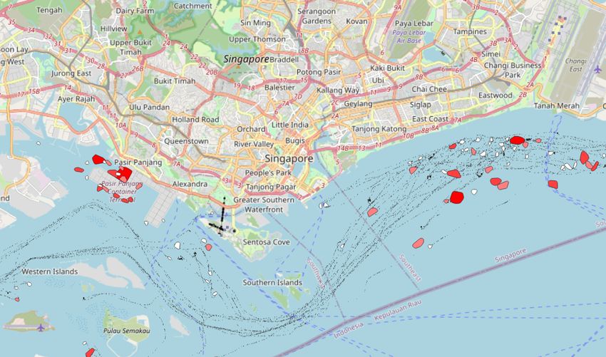
2

of vessels at ports. Existing solutions to the port classification problem generally focus on
analyzing static features of actual ports, lacking a temporal aspect. An effective solution to
port classification problem needs to take into account spatio-temporal dependencies of the
underlying data. While Graph Neural Networks (GNNs) enable modeling such spatial rela-
tions, dynamic graphs enable encoding temporal changes in the graph structure encountered
over time, such as the addition or removal of nodes or edges.

        Figure 1. The illustration of the extracted actual and gateway ports from AIS data
        based on visiting frequencies. The gateway ports are clustered on the right side with
        close proximity to actual ports.

   In this paper, we propose a Temporal Graph Neural Network (TGNN) based method
for maritime port classification. The graph representation makes it possible to capture
underlying spatial relations, and the proposed method processes the information encoded in
the graphs temporally to capture temporal dependencies. A time-ordered graph sequence
is constructed from the automatic identification system (AIS) data which contains logs
obtained from vessels as they sail. The graph is built by partitioning the AIS data into
blocks where each block corresponds to a period of time (i.e., daily, weekly). The resulting
graph sequence is processed temporally to classify ports. The proposed method is evaluated
on real-world AIS data in terms of its effectiveness of correctly classifying ports. The
experimental results show that the proposed method classifies ports with an f-score of 95%.
   The contributions of this study are three-fold:
     • We propose a novel dynamic graph representation for the port classification problem,
       capturing spatio-temporal relations between various dynamic and static features of
       vessel trajectories.
     • We develop a novel TGNN-based method for discovering gateway ports and classi-
       fying target ports as either actual or gateway ports.
     • We experimentally demonstrate the effectiveness of the proposed method on a real-
       world data set, showing the classification performance in terms of precision, recall
       and f-score.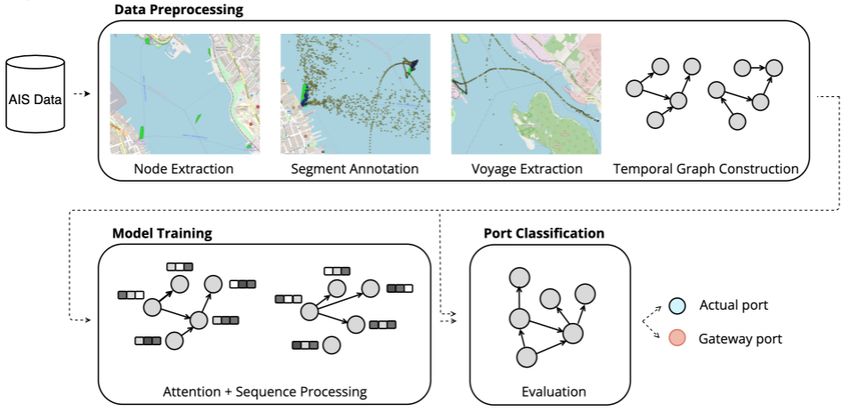
3

    This paper is organized as follows: First, the literature of the described problem is
presented. Then, the related notations on the maritime port classification are given. This
is followed by the explanation of the proposed port classification method. Afterwards, the
evaluation of the proposed method is presented on real-world AIS data. Finally, the paper
is concluded with potential future directions.

2. Related Work

   In this section, we first review existing studies on port classification problem. Then,
we briefly present approaches addressing node extraction, which is an auxiliary task in our
research.

2.1. Port classification studies

    Several studies are presented to classify ports considering various port features [6–9]. Roa
et al. [6] classify ports by their sizes and facility types to find out the applicable business
models for corresponding types of ports. Another example is Malaysian ports which are
classified based on port characteristics such as port size, traffic, and infrastructure [7].
Similarly, Nguyen et al. [8] classify dry ports, which are inland terminals where customers
load/unload cargo, considering features such as development reasons, roles, etc. Park and
Medda [9] present a port classification scheme for container ports considering inland and
shipping networks to investigate the economic relationship between ports and their regions.
Such existing studies follow qualitative approaches and do not concern with the spatio-
temporal data collected from vessels.
    Clustering methods are used in the literature to classify ports. Azzam et al. [10] present
a multi-level k-means clustering approach to cluster and classify ports considering their
properties such as harbor type and size. Another work by Mansouri et al. [11] considers
k-means clustering to cluster ports taking into account port features such as port size and
annual throughput. Such solutions only take into account physical properties of ports while
lacking the temporal aspect of the problem.
    A recent study by Carlini et al. [12] proposes an AIS data representation where the model
is adapted from a Global Shipping Network (GSN) structure, with vertices corresponding to
ports and edges corresponding to the connections (i.e., voyages) between the ports. In that
particular study, the authors show that the movement patterns of some specific types of
vessels, such as short-range vessels, change over time due to seasonal trends. Consequently,
a temporal analysis of AIS data is crucial. Different from earlier port classification studies,
first, we discover gateway ports, which are waiting regions. Second, we classify actual and
gateway ports in the maritime domain by considering not only the spatial but also the
temporal dependencies of the processed vessel trajectory data.

2.2. Node extraction studies

   Vessel navigation movement is accessible in the form of a trajectory which is a series of
consecutive spatio-temporal data. Prepossessing such data is required to form the proper
inputs for our TGNN model. There are many studies with the focus of finding stop points in
a trajectory such as stay point detection [13], stops and moves of trajectories (SMOT) [14],
clustering-based stops and moves of trajectories (CB-SMOT) [15], and direction-based stops
and moves of trajectories (DB-SMoT) [16]. These algorithms are categorized as part of
trajectory segmentation studies where a trajectory is segmented based on a specific criteria.
The utilization of the density-based spatial clustering of applications with noise (DBSCAN)
algorithm [17] as one of the core algorithms is notable in these studies.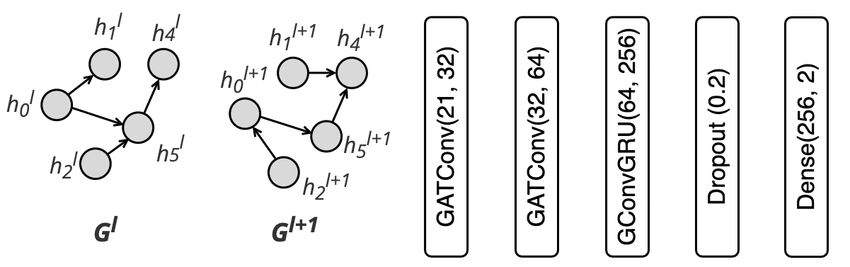
4

3. Notations

    This section describes the notations relevant for the maritime port classification problem
addressed in the paper.
AIS message. Vessels transmit messages and log their movements during the voyages,
which are called AIS messages. Formally, we define each vessel with s and an AIS message
is denoted as a tuple, m = (x, y, t, s, sog) where x and y denote GPS coordinates as degrees
for longitude and latitude in the EPSG:4326 Geodetic system. t denotes the timestamp
of the message, and sog denotes speed over ground, respectively. The entire set of AIS
messages is denoted with M .
Port. Vessels navigate in the sea between points, and these points are called ports. A port
p is represented as a tuple (id, x, y) where id corresponds to the unique identifier of the
port and x and y denote the center of the GPS coordinates as degrees for longitude and
latitude in the EPSG:4326 Geodetic system. We also consider a spatial function γ(p, c),
which specifies a polygon as the port region with an ordered sequence of point sequences
c that defines the corresponding polygon, and it is centered on coordinates of the specific
port p. The global set of ports are denoted as p ∈ P .
Trajectory. Vessels follow a series of points (coordinates) in the sea and these time-ordered
consecutive coordinates make up the trajectory of that particular vessel. In this study, we
represent a trajectory of a vessel s with trs = ((x, y)0 , (x, y)1 , ..., (x, y)n ) where (x, y) is a
binary tuple that includes degrees for longitude and latitude.
Visit. Vessels navigate and visit ports to fulfill their business objectives. We explicitly
define a visit v = (p, m, t) of the vessel s to a port p at time t with the condition that there
is at least one m ∈ M with coordinates x and y in the port area given by γ(p, c) considering
the ordered points c that define the port.
Voyage. Two consecutive visits to different ports are considered voyages, and it is denoted
as a pair of visits voy = (v1 , v2 ) and the same vessel performed both visits (v1 (s) = v2 (s)).
One should also note that these visits need to be consecutive in terms of time (v1 (t) < v2 (t)),
and there should be no visits to other ports performed by the corresponding vessel between
v1 (t) and v2 (t). The ports of v1 and v2 satisfying these criterion are called origin and
destination ports, respectively.

4. TGGN-based Port Classification Approach

   Our proposed approach to maritime port classification is based on Temporal Graph Neural
Networks (TGNNs). In this section, we first present preliminaries of the TGNN structure,
then elaborate on the proposed port classification approach.

4.1. Temporal Graph Neural Networks (TGNNs)

   A graph neural network (GNN) is represented with G = (V, E) where V is the vertex
set and E is the edge set of the graph G. In a GNN, information is embedded into nodes
and edges to come up with inferences. Each node is denoted with hi ∈ V , and each edge is
denoted with eij where i and j denote node indices. Consecutive graphs ordered by time
make up a TGNN, and it includes layers, each of which is denoted with l corresponding to a
distinct time step. Information is encoded into the nodes and edges in this temporal graphs.
Node encodings correspond to enc(hli ) where l is the layer index and i is the node index
in the corresponding graph layer. Edge encodings correspond to enc(elij ) where l is the
layer index and i and j denote the corresponding node indices. Node-level, edge-level and
graph-level inferences are possible by taking into account node and edge encodings. In this
particular study, we adopt a node-level prediction method to classify ports. The upcoming
section presents the details of how we adapt this formulation for our TGNN-based method.
5
4.2. The Proposed Algorithm
The dynamic graphs underlying our TGNN consist of nodes (V ) as ports (P ). A node
encoding at the layer l (enc(hli )) corresponds to the features tailored from port information
and the AIS message set (M ). An edge encoding at the layer l (enc(elij )) corresponds to the
distances between the corresponding ports (δ(pi , pj ) where δ is haversine distance function
and i and j are port indices).
Our proposed TGNN-based method includes three stages: data preprocessing, model
training and port classification. Tasks such as node extraction, segment annotation, voyage
extraction and temporal graph construction are performed in the data preprocessing stage.
This is followed by the model training stage where temporal graphs are used to train a TGNN
model. The final stage is port classification, and the trained model is used to classify ports
with the labels actual and gateway ports.
Figure 2. The stages of the proposed port classification algorithm.
Figure 2 illustrates the stages of the proposed port classification method. First, ports are
extracted from the log messages obtained from vessels, AIS data (node extraction). Then,
each AIS message is annotated, whether it is a message obtained while the vessel was within
a port region or on the sea (segment annotation). Later, voyages of vessels are extracted (i.e.,
the start and end ports of the vessels) in the voyage extraction stage. Afterwards, the input
data is represented as a sequence of graphs (temporal graph construction). Finally, a model
is trained for the port classification task, and it is evaluated. The upcoming subsections
elaborate the details of these tasks.
Node Extraction. The aim of the node extraction task is to extract ports from the AIS
data. We use DBSCAN algorithm to extract ports. DBSCAN has two parameters: epsilon
(eps) and the minimum number of points in each cluster (minP ts). We experiment with
different values for these parameters, and our experiments show that using minP ts = 20
and eps = 0.005 degree which is near to 500 meters is a reasonable decision and can identify
nodes that are more relevant to a subject matter expert. We use spatial operation and
PostGIS to keep a set of nodes and merge newly discovered ports using a buffered convex-
hull of the adjacent port and the newly discovered port.
Segment Annotation. After the node extraction task, the segment annotation task takes
place. This task aims to label all AIS messages m ∈ M that include trajectory points (x, y)6
with the following labels: id or seapoint. The label id indicates that the corresponding
trajectory point falls into a port region that is extracted in the previously described node
extraction task, and its label is the id of that particular port. If a trajectory point is not
located within any of the extracted ports, then it is annotated with the label seapoint.
Formula 4.1 formulates this segmentation task as a partial function.
(
pj .id ∃pj (mi .(x, y) ∈ γ(pj , cj ))
label(mi ) = (4.1)
seapoint otherwise
Voyage Extraction. Voyage extraction task requires investigating the annotated trajec-
tory points to extract voyages. This necessitates keeping track of the ordering of segment
annotations. To exemplify, once an AIS message that contains an id as its label is encoun-
tered, the corresponding port with that id is considered as the source of the voyage (vi ).
Then, this voyage is tracked until another AIS message with an id as its label is encountered
after a number of sequential seapoint labels. This port is then considered as the destination
of the corresponding voyage (vj ), and the voyage voy = (vi , vj ) is registered as a new voyage.
Temporal Graph Construction. After the voyages are extracted from the AIS data, the
temporal graph construction task takes place. For each pre-defined time interval, a graph
Gl is generated with the information encoded on it. In this study, we take the time interval
a single calendar day and generate daily graphs. We empirically set this interval to a single
calendar day as the used data set for the evaluation includes AIS messages of passenger
vessels operating between ports located within proximity. Port-related information is en-
coded in the nodes (enc(hli )) for the corresponding day as we associate ports with nodes in
our representation. The following features extracted from AIS messages are embedded in
the nodes: port visit frequencies, waiting times in the ports, and port arrival average speed
statistics. This information is concatenated to form a vector that represents node features
for each node. Considering the taxonomy presented by Rozemberczki et al. [18] to represent
spatiotemporal input data, our design falls into the category dynamic graph with temporal
signal as both the graph structure (i.e., addition/removal of nodes/edges) and the node
features (i.e., the embedded information on nodes) change at each time step. The following
items elaborate on each tailored feature.
• Port visiting statistics: This feature corresponds to the visiting statistics of ports
by the vessels within a period of time. This information is extracted for each port
taking into account the number of arrivals and departures of vessels to and from
that particular port. This statistic is calculated separately as a voyage may start
and end on different calendar days.
• Waiting time: This feature corresponds to the vessels’ existence times in port regions
for a given period of time in terms of minutes.
• Speed statistics: This feature corresponds to the average speeds of vessels during
the voyages. We extract this feature for each port. We also consider average speeds
of vessels while they are in a port region.
As edges are associated with the connectivity of ports (i.e., there is at least one voyage
between the ports pi and pj occurred on a day corresponding to the layer l on the graph),
we utilize the haversine distance between the nodes as edge encodings (enc(elij )). At the end
of the temporal graph generation task, a time-ordered temporal graph sequence is obtained
with the node embeddings as port-related features, and edges as the adjacency relations
(i.e., the distance between ports).
To learn and capture underlying patterns in the AIS data, we use a TGNN design which
is depicted in Figure 3. We employ two attention-enabled graph convolution layers, namely
GATConv [19]. Each convolution layer includes two attention heads with a mean aggregation
scheme for message passing, and the edge dimension is set to one. These convolution layers7
Figure 3. The designed TGNN for the port classification problem.
are followed by a recurrent graph convolution layer that builds on gated recurrent units
(GRUs), namely, GConvGRU [20]. The graph sequence is processed in this layer and the
result is fed into a dropout layer. Later on, a dense layer is employed which is followed by
a softmax layer to map the input to classes.
5. Experimental Evaluation
This section presents the experimental setup followed by the experimental results answer-
ing the three research questions. We evaluate the proposed method in terms of its capability
and robustness on a real-world dataset. Specifically, we are interested in answering the fol-
lowing research questions:
RQ1 Is the model effective in classifying maritime ports?
RQ2 How do the spatio-temporal relations affect the port classification performance?
RQ3 Is the model robust under different configuration changes, i.e., different dropout
probabilities as a regularization parameter?
5.1. Experimental Setup
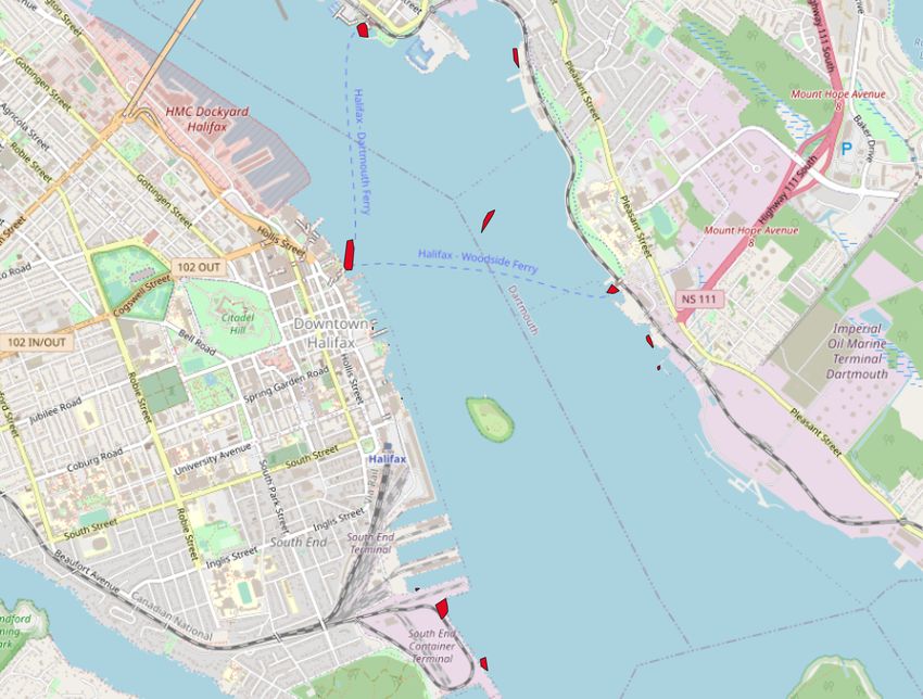
Dataset. We use a publicly available1 real-world data set to evaluate our presented port
classification method. The dataset includes 513012 AIS messages obtained from 10 vessels
operating within a port region of Halifax, NS, Canada between March 2019 and July 2019,
shown in Figure 4. There is a total of 15 ports extracted, and for the sake of space, only 10
ports are shown in the figure.
Evaluation metrics. We first evaluate the performance of the proposed method in
terms of its effectiveness in accurately classifying ports by presenting confusion matrices.
Then, we analyze the classification performance with respect to the following classification
scores: precision, recall and f-score. Finally, we evaluate changes of training and validation
losses during the training.
Training. We train our model to learn a total number of 500066 trainable parameters.
We use time series split cross validation to validate our model, and we partition the data
by taking into account the time dimension of the input graph sequence. We set the number
of split as eight. An early stopping scheme is applied to decide on when to stop training.
It considers the validation loss with an empirically set patience threshold. To tackle the
imbalanced class distribution in the data set, we use adaptive weights while updating the
model’s parameters during training; that is, the more instance a class has, the less weight
it has. We utilize PyTorch for model implementation and PyTorch Geometric Temporal
library [18] for processing spatio-temporal data. Table 1 lists the parameters that are used
during training.
1https://github.com/metemaad/WS-II8
Figure 4. The port region of Halifax used in the experiments. Red regions denote the
extracted ports.
Table 1. Hyperparameters that are used during training phase.
Parameter Value
Optimizer Adam
Loss Cross Entropy
Learning rate (η) 10−4
Dropout 0.2
Patience 10
5.2. Experimental Results and Analysis
5.2.1. Classification Effectiveness
Figure 5 presents the normalized confusion matrices of the proposed method for the
different settings. Vertical axes denote the actual labels, and horizontal axes denote the
predicted labels by the method. The first confusion matrix (Figure 5a) depicts the classifi-
cation performance of the proposed method where a temporal analysis on the input graphs
is excluded (i.e., the graphs are processed individually without any propagation of temporal
information). The second confusion matrix (Figure 5b) depicts the results of the setting
where the attention-enabled graph convolution layers are excluded in the design. The last
confusion matrix (Figure 5c) depicts the obtained results with the proposed method where
consecutive input graphs are processed, taking into account the temporal dimension, and
activating the attention-enabled graph convolution layers.
As can be seen from Figure 5a, when temporal analysis is excluded, the method predicts
only 54% of the ports accurately, while it predicts 56% of the gateway ports accurately.
Considering the results in Figure 5b, excluding only attention yields to predicting 94%
of the ports accurately. This setting also provides an improvement in predicting gateway9
(a) (b) (c)
Figure 5. The normalized confusion matrices for (a) the TGNN method w/o temporal
analysis (b) w/o attention (c) w/ both temporal analysis and attention.
ports with a score of 88%. Incorporating attention and temporality together provides a
classification score of 91% for ports, which is less than 3% compared to the previous setting.
On the other hand, this setting provides a 96% classification score for the gateway ports,
which is 8% more than the setting where the attention mechanism is excluded.
Table 2. Performance analysis of the proposed method with different settings.
Precision Recall F-Score
α t µ±σ µ±σ µ±σ
X 0.90 ± 0.02 0.55 ± 0.16 0.59 ± 0.14
X 0.97 ± 0.04 0.93 ± 0.07 0.94 ± 0.06
X X 0.98 ± 0.02 0.93 ± 0.05 0.95 ± 0.06
5.2.2. Effect of Spatio-temporal Relationships
Table 2 presents the classification scores in terms of precision, recall and f-score. Each
row presents the weighted scores of a distinct setting, and each column presents the score
for the corresponding metric. α denotes whether attention is used, and t stands for whether
a temporal analysis is applied to the input. As can be seen from the table, the setting where
only attention is used provides an f-score of 59%. On the other hand, the setting where only
temporality is used provides an f-score of 94%, which is significantly better than the previous
setting where only attention is used. When attention and temporality are incorporated, a
slight performance improvement is achieved with an f-score of 95%. In our representation,
temporality enables the graph sequence to propagate information between graph instances
through time. Attention enables the nodes that correspond to ports to be aware of their
neighbor ports by considering their attention scores. Considering the misclassified instances,
those settings where attention or temporality is excluded confuse labels most of the time
when the graph constructed for that corresponding day is sparse (i.e., there are isolated
nodes in the graph which means some ports are not visited during that day). In such
graphs, the spatio-temporal relationships are fewer.
5.2.3. Classification Robustness to Configuration Changes
To avoid overfitting and make the model generalize better, we use dropout and early
stopping as regularization techniques. Table 3 presents the effect of the dropout probability
choice on the performance. Each row presents the results of a different dropout probability
setting, and each column presents the scores of a distinct metric. First, we analyze the case10
where the dropout layer is disabled. This setting provides an f-score of 0.89 as a baseline.
When the dropout probability is set to 0.1, an f-score of 0.94 is achieved. Setting the dropout
probability to 0.2 provides the best result with an f-score of 0.95. As the dropout probability
is set to 0.3, the obtained f-score drops to 0.92. In our experiments, we choose the setting
where the dropout probability is 0.2 as it provides the best f-score.
Table 3. Performance analysis of the proposed method for different dropout probabilities.
Precision Recall F-Score
Probability µ±σ µ±σ µ±σ
0 0.97 ± 0.04 0.86 ± 0.07 0.89 ± 0.05
0.1 0.97 ± 0.02 0.91 ± 0.09 0.94 ± 0.07
0.2 0.98 ± 0.02 0.93 ± 0.05 0.95 ± 0.06
0.3 0.97 ± 0.02 0.91 ± 0.08 0.92 ± 0.06
Figure 6. Training and validation loss. Early stopping scheme stops training when the
validation loss starts to increase.
Figure 6 presents an analysis on training and validation loss during the model training
phase. The y-axis denotes the loss, and the x-axis stands for the epoch number. The red line
indicates the training loss and the blue line indicates the validation loss. In this particular
training instance, the validation loss starts to increase around epoch 270. At this point, we
stop the training and select the target model for evaluation.
6. Discussion and Conclusion
This research addresses a significant problem in the maritime domain, which is the port
classification problem. It deals with discovering gateway ports (which are not actual ports
but waiting regions for vessels) and distinguishing between gateway and actual ports. To
this end, we present a novel TGNN-based port classification method that processes spatio-
temporal AIS data. The proposed method first extracts ports from the raw AIS data then
annotates segments in the AIS messages. Later, the voyages are extracted, taking into
account the extracted port information and the segment annotations. This is followed by
constructing a time-ordered daily graph sequence encoded with these extracted features.
The performance of the proposed method is evaluated on a real-world data set consisting of11
logs collected from vessels sailing in Halifax, NS, Canada, in terms of precision, recall and
f-score. The conducted experiments show that our TGNN-based port classification method
has the ability to effectively classify maritime ports by taking into account spatio-temporal
dependencies of the underlying data with an f-score of 95%. Furthermore, the experiments
demonstrate that excluding attention (which evaluates the importance of neighboring ports
as a spatial analysis) or temporal analysis from the proposed method yields degraded per-
formance.
We believe that this study fills a gap in the literature by bringing up the discovery of
gateway ports and distinguishing them from actual ports. The preliminary obtained results
are promising in terms of the achieved classification scores on the available real-world AIS
data set. We are aware of the fact that the data set used in the experiments is limited in
terms of the number of considered ports. It is worth to note that one of the main challenges
of the port classification problem is the lack of available benchmark data sets annotated
with the ground truth. Therefore, we believe this study presents an important initial step
for the discovery of gateway ports and classifying gateway and actual ports. We leave the
investigation of the port classification problem with a more extensive number of ports located
in different regions and a more comprehensive comparative analysis with other baselines as
future work. We also plan to process the detected gateway port information to optimize
vessel trajectories by applying graph optimization algorithms.
Acknowledgements
This work is supported by ECSEL JU under grant agreement No 101007260 and the
Research Council of Norway under grant agreement No 329090.
References
[1] U. N. C. on Trade and Development. Review of Maritime Transport 2018. United Nations,
2018. url: https://www.un-ilibrary.org/content/books/9789210472418.
[2] D. S.-H. Moon and J. K. Woo. “The impact of port operations on efficient ship operation
from both economic and environmental perspectives”. In: Maritime Policy & Management
41.5 (2014), pp. 444–461.
[3] A. Alessandrini, F. Mazzarella, and M. Vespe. “Estimated time of arrival using historical vessel
tracking data”. In: IEEE Transactions on Intelligent Transportation Systems 20.1 (2018),
pp. 7–15.
[4] K. Park, S. Sim, and H. Bae. “Vessel estimated time of arrival prediction system based on a
path-finding algorithm”. In: Maritime Transport Research 2 (2021), p. 100012.
[5] A. Agra, M. Christiansen, A. Delgado, and L. M. Hvattum. “A maritime inventory routing
problem with stochastic sailing and port times”. In: Computers & Operations Research 61
(2015), pp. 18–30.
[6] I. Roa Perera, Y. Peña, B. Amante García, and M. Goretti. “Ports: Definition and study
of types, sizes and business models”. In: Journal of industrial engineering and management
(JIEM) 6.4 (2013), pp. 1055–1064.
[7] M. K. Othman, N. S. F. A. Rahman, A. Ismail, and A. Saharuddin. “The sustainable port
classification framework for enhancing the port coordination system”. In: The Asian Journal
of Shipping and Logistics 35.1 (2019), pp. 13–23.
[8] C. Nguyen et al. “Dry ports as extensions of maritime deep-sea ports: a case study of Vietnam”.
In: Journal of International Logistics and Trade 14.1 (2016), pp. 65–88.
[9] Y.-A. Park and F. Medda. “Classification of container ports on the basis of networks”. In:
Proceedings of 12th World Conference on Transport Research (WCTR), Lisbon, Portugal
(2010), pp. 1–17.
[10] I. A. Azzam, S. F. Al-Khatib, and W. M. Albataineh. “Strategic port classification: Inter-
national clustering-based approach for decision-making optimization”. In: Journal of Public
Affairs 21.1 (2021), e1963.12
[11] F. S. Mansouri, A. Allal, K. Mansouri, and M Qbadou. “A model for analyzing capacity
of ports to accommodate autonomous ships using k-means cluster analysis: a case study”.
In: International Journal on Technical and Physical Problems of Engineering 13.2 (2021),
pp. 68–75.
[12] E. Carlini, V. M. de Lira, A. Soares, M. Etemad, B. Brandoli, and S. Matwin. “Understanding
evolution of maritime networks from automatic identification system data”. In: GeoInformat-
ica (2021), pp. 1–25.
[13] Y. Zheng, L. Zhang, Z. Ma, X. Xie, and W.-Y. Ma. “Recommending friends and locations
based on individual location history”. In: ACM Transactions on the Web (TWEB) 5.1 (2011),
p. 5.
[14] L. O. Alvares, V. Bogorny, B. Kuijpers, J. A. F. de Macedo, B. Moelans, and A. Vaisman.
“A model for enriching trajectories with semantic geographical information”. In: Proceedings
of the 15th annual ACM international symposium on Advances in geographic information
systems. 2007, pp. 1–8.
[15] A. T. Palma, V. Bogorny, B. Kuijpers, and L. O. Alvares. “A clustering-based approach for
discovering interesting places in trajectories”. In: Proceedings of the 2008 ACM symposium
on Applied computing. 2008, pp. 863–868.
[16] J. A. M. R. Rocha, V. C. Times, G. Oliveira, L. O. Alvares, and V. Bogorny. “DB-SMoT:
A direction-based spatio-temporal clustering method”. In: 2010 5th IEEE International Con-
ference Intelligent Systems. 2010, pp. 114–119. doi: 10.1109/IS.2010.5548396.
[17] M. Ester, H.-P. Kriegel, J. Sander, X. Xu, et al. “A density-based algorithm for discovering
clusters in large spatial databases with noise.” In: kdd. Vol. 96. 34. 1996, pp. 226–231.
[18] B. Rozemberczki, P. Scherer, Y. He, G. Panagopoulos, A. Riedel, M. Astefanoaei, O. Kiss, F.
Beres, G. López, N. Collignon, et al. “Pytorch geometric temporal: Spatiotemporal signal pro-
cessing with neural machine learning models”. In: Proceedings of the 30th ACM International
Conference on Information & Knowledge Management. 2021, pp. 4564–4573.
[19] P. Veličković, G. Cucurull, A. Casanova, A. Romero, P. Lio, and Y. Bengio. “Graph attention
networks”. In: arXiv preprint arXiv:1710.10903 (2017).
[20] Y. Seo, M. Defferrard, P. Vandergheynst, and X. Bresson. “Structured sequence modeling with
graph convolutional recurrent networks”. In: International Conference on Neural Information
Processing. Springer. 2018, pp. 362–373.You can also read