DISCUSSION PAPER SERIES - Gender Differences in Reference Letters: Evidence from the Economics Job Market - Institute of ...
←
→
Page content transcription
If your browser does not render page correctly, please read the page content below

DISCUSSION PAPER SERIES

IZA DP No. 15055

Gender Differences in Reference Letters:
Evidence from the Economics Job Market

Markus Eberhardt
Giovanni Facchini
Valeria Rueda

JANUARY 2022

DISCUSSION PAPER SERIES

IZA DP No. 15055

Gender Differences in Reference Letters:
Evidence from the Economics Job Market

Markus Eberhardt
University of Nottingham and CEPR
Giovanni Facchini
University of Nottingham, CEPR and IZA
Valeria Rueda
University of Nottingham and CEPR

JANUARY 2022

Any opinions expressed in this paper are those of the author(s) and not those of IZA. Research published in this series may
include views on policy, but IZA takes no institutional policy positions. The IZA research network is committed to the IZA
Guiding Principles of Research Integrity.
The IZA Institute of Labor Economics is an independent economic research institute that conducts research in labor economics
and offers evidence-based policy advice on labor market issues. Supported by the Deutsche Post Foundation, IZA runs the
world’s largest network of economists, whose research aims to provide answers to the global labor market challenges of our
time. Our key objective is to build bridges between academic research, policymakers and society.
IZA Discussion Papers often represent preliminary work and are circulated to encourage discussion. Citation of such a paper
should account for its provisional character. A revised version may be available directly from the author.

                                                     ISSN: 2365-9793

                                           IZA – Institute of Labor Economics
Schaumburg-Lippe-Straße 5–9                      Phone: +49-228-3894-0
53113 Bonn, Germany                             Email: publications@iza.org                                    www.iza.org
IZA DP No. 15055                                                                                                             JANUARY 2022

            ABSTRACT
            Gender Differences in Reference Letters:
            Evidence from the Economics Job Market*
            Academia, and economics in particular, faces increased scrutiny because of gender
            imbalance. This paper studies the job market for entry-level faculty positions. We employ
            machine learning methods to analyze gendered patterns in the text of 9,000 reference
            letters written in support of 2,800 candidates. Using both supervised and unsupervised
            techniques, we document widespread differences in the attributes emphasized. Women are
            systematically more likely to be described using “grindstone” terms and at times less likely
            to be praised for their ability. Given the time and effort letter writers devote to supporting
            their students, this gender stereotyping is likely due to unconscious biases.

            JEL Classification:              J16, A11
            Keywords:                        gender, natural language processing, stereotyping, diversity

            Corresponding author:
            Valeria Rueda
            School of Economics
            Sir Clive Granger Building
            University of Nottingham
            University Park
            Nottingham NG7 2RD
            United Kingdom
            E-mail: valeria.rueda@nottingham.ac.uk

            * We gratefully acknowledge financial support from STEMM-CHANGE, University of Nottingham and Econ Job
            Market for authorizing the use of the data. Malena Arcidiácono, Cristina Griffa, Yuliet Verbel-Bustamante, Thea
            Zoellner, and Diego Marino-Fages have provided excellent research assistance. The views expressed in this paper are
            those of the authors and do not necessarily represent the views of the University of Nottingham. We thank seminar
            participants at Bocconi University and the Monash-Zürich text-as-data conference for their comments.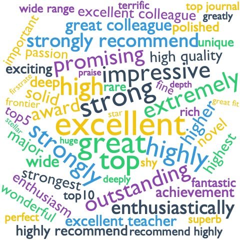
1       Introduction
Gender disparities in the workplace have received significant attention in public debate.
Academia is facing increased scrutiny due to its low female representation (Valian, 1999),
especially in the field of economics (Lundberg, 2020, Part I). Recent empirical work has doc-
umented that the economics career pipeline for women is “leaky”, meaning that women tend
to drop out of the profession at critical transitions, such as the jump from earning a Ph.D. to
an assistant professorship, or from assistant to associate professor (for a broad review, see
Lundberg and Stearns, 2019). This paper studies the first step of the academic career of an
economist, the junior “job market” —the stage at which the leak has grown the most in the
past decade (Lundberg and Stearns, 2019)— and which so far has not received much sys-
tematic attention (Lundberg, 2020).1

The academic job market in economics is unique in that it is a highly structured institution. It
starts every year in late Fall with universities posting their job advertisements and potential
applicants preparing a “job market package”. The latter consists of one or more academic
papers, a CV and a set of recommendation letters written by scholars familiar with the candi-
date. All the parties involved, i.e. the candidates, the letter writers and the hiring committees,
interact via centralized platforms. Typically, the same package is used for the vast majority
of jobs, making the marginal cost of an additional application low. Reference letters are not
tailored to a particular institution and the same letter is usually used for all job applications
(for more details see Coles et al., 2010).

In this paper, we investigate the presence of differences in the language used in reference let-
ters, depending on the gender of the candidate being recommended. We use a unique dataset
encompassing all applications for entry level positions received by a research-intensive uni-
versity in the U.K. over the 2017-2020 period. Deploying Natural Language Processing tools,
we analyze the text of over 9,000 reference letters written in support of 2,800 candidates. A
standard letter covers a lengthy discussion of the candidate’s job market paper, some refer-
ence to their additional research, and to their teaching and citizenship skills. Importantly,
the final section of the letter provides a summary assessment of the candidate’s academic
abilities and recruitment prospects. Since we are primarily interested in the way candidates
are described, we primarily focus on this final section. This corpus is then transformed into a
term-frequency-inverse-document-frequency (tf-idf) representation. Borrowing from meth-
ods developed in cognitive psychology and linguistics, we quantify whether letters written
in support of female candidates emphasize systematically different attributes.

We use two complementary approaches. First, we employ an unsupervised methodology to
ascertain the terms in the letters that are the best predictors of a candidate’s gender. We adopt
a LASSO technique that selects the strongest predictors. Among these, we frequently ob-
serve terms related to research interests, but also to personality and “grindstone” attributes
    1
   There is work on this issue in other disciplines, see for example Madera et al. (2009); Dutt et al. (2016);
Hebl et al. (2018).

                                                      2
(“determined”, “diligent”, “hardworking”, etc.). Second, we rely on a supervised method,
building dictionaries of words for common attributes emphasized in reference letters. These
dictionaries are informed by existing research on the topic (Trix and Psenka, 2003; Schmader
et al., 2007). We validate our dictionaries through an original comprehensive survey of
academic economists based in U.K. research-intensive universities. Corroborating the ex-
ploratory results from the LASSO, we observe that descriptions of female candidates tend
to emphasize significantly more “grindstone” attributes. In further specifications, we also
uncover a tendency to use fewer terms related to ability.

Diligence and working hard are positive attributes (see Alan et al., 2019, on ‘grit’). However,
given the overwhelmingly positive tone of recommendation letters in the job market, it may
be misleading to interpret our findings as suggesting that women receive ‘better’ recommen-
dations. The opposite may well be true. In fact, as noted by Valian (1999, p. 170) “[a]lthough
working hard is a virtue, labeling a woman a hard worker can be damning with faint praise.
If someone is not considered able to begin with, working hard can be seen as confirmation of
his or her inability.” More generally, sociologists have pointed out that minorities are more
often praised for their diligence than for their innate ability and that the signal of diligence
is often interpreted as a lack of innate talent (Bourdieu and Passeron, 1977, p.201).

In additional results, we also find that female candidates are on average weakly and insignifi-
cantly associated with more teaching and citizenship terms, but this pattern hides important
heterogeneities. In mid-ranking departments, the effect is strongly positive and significant
whereas the opposite is true for elite institutions. We observe a similar pattern for the us-
age of standout terms. All our results are robust to a variety of specifications and across
multiple relevant subsamples (e.g. depending on geographical location or institutional rank-
ing).

We expect differences in the language of reference letters to depend on many factors, such as
the institution the candidate graduated from or their research field. Some of these determi-
nants may differ systematically for male and female candidates. We tackle this problem in a
variety of ways.

In our baseline specifications we control for observable candidate and writer characteristics
obtained from the application platform and from additional information we collected man-
ually. On the writer’s side, we control for their gender, the number of letters they provide in
our sample, and the ranking of their institution. On the candidate’s side, we control for their
ethnicity, years since Ph.D. completion, broad field of specialization, publication record, and
the ranking of their Ph.D.-awarding institution. The baseline results are not very sensitive to
these controls, nor to alternative definitions of the reference letter ends.

Still, we may worry that unobservable determinants could affect our findings. We therefore
run more restrictive models that allow us to account for unobserved, time-invariant insti-
tutional and letter-writer characteristics. A first set of models, which include fixed effects

                                               3
for the Ph.D.-granting institution, confirm the gendered patterns observed even for candi-
dates of the same cohort at the same institution. In further analysis, we restrict the sample
to referees who have written letters for both male and female candidates and employ writer
fixed effects. These more demanding specifications confirm that differences in describing
male and female candidates are detectable even when we focus on individual writers. Fur-
ther probing indicates that more experience writing for female candidates attenuates some
of these differences.

This article is related to the literature on gender representation in academia. Several pa-
pers have shown that women are under-represented in math-intensive fields (for a detailed
review of the literature see Ceci and Williams (2009, p.3-16), Kahn and Ginther (2017)).
Investigations of different aspects of academic life have uncovered significant barriers. For
example, Nittrouer et al. (2018) and Hospido and Sanz (2021), among others, observe that
female academics are less likely to be accepted to present their work at academic conferences.
Many researchers have emphasized systematic gender biases in student evaluations of teach-
ers, which are frequently-used indicators of performance in promotion and tenure packages
(MacNell et al., 2015; Boring, 2017; Fan et al., 2019; Mengel et al., 2019; Boring and Philippe,
2021).

While other math-intensive fields have shown some improvement, Economics has been in
the spotlight for its persistently low representation of women (Bayer and Rouse, 2016; Lund-
berg and Stearns, 2019). Not only is there low female representation at the earliest stages
of the profession, but the career pipeline is also “leaky”. In trying to understand barriers
to women’s advancement in Economics, researchers have looked at different stages of an
academic career. Focusing on the first one, Boustan and Langan (2019) document the wide
variation of gender representation across Ph.D. programs, and that this representation tends
to be a persistent attribute of a department. They also observe that for U.S. placements, men
on average land jobs in higher-ranked institutions. Turning to the next steps as academic
professionals, other limitations to the advancement of women have been observed. In par-
ticular, there is evidence that females face barriers to promotion (Ginther and Kahn, 2004;
Sarsons, 2017; Bosquet et al., 2019), higher standards to judge the quality of their research
(Card et al., 2020; Dupas et al., 2021; Grossbard et al., 2021; Hengel, forthcoming), and that
their work gets cited less (Koffi, 2021). Taken together, all these factors are likely to ham-
per the progression of women in their academic careers. We contribute to this burgeoning
literature by focusing on a major and to date unexplored stepping stone: the junior job mar-
ket. At this stage, beyond institutional credentials, little information about the candidate’s
research or teaching is observed. Therefore, reference letters play a crucial role in supporting
the applicant.

The professional culture in Economics may also be problematic for women’s advancement.
Wu (2018) reports evidence of gender biases in posts about women in a well-known and
widely used anonymous forum in the profession. Similarly, Dupas et al. (2021) study the

                                               4
seminar culture and present evidence that female speakers face more hostile audiences. By
analyzing recommendation letters, we are investigating a different aspect of the professional
culture, namely mentorship. As opposed to these previous studies, our focus is on a setting
in which economists fulfil a supportive and nurturing role.
We also contribute to the literature carrying out text analysis in academic recommendation
letters (Trix and Psenka, 2003; Schmader et al., 2007; Dutt et al., 2016; Hebl et al., 2018; Madera
et al., 2019). We build on this earlier work to classify the types of attributes usually empha-
sized in these letters. Additionally, to the best of our knowledge, we are the first to vali-
date our classification by surveying a large sample of academics. Moreover, focusing on eco-
nomics, we can access a substantially larger sample of letters that are broadly representative
of a highly structured and globalized academic job market.
The paper is organized as follows. In Section 2 we discuss our sample as well as the gen-
eral approach of our main textual analysis. Section 3 explains the process of data cleaning
and preparation, followed by the exploratory analysis using unsupervised methods in Sec-
tion 4. Section 5 outlines the supervised approach and presents the baseline results, with
extensions and additional robustness checks provided in Section 6, followed by concluding
remarks.
2 Data
We collected and cleaned the text of over 9,000 reference letters written in support of 2,800
candidates who applied for entry-level positions between 2017 and 2020 at a research inten-
sive economics department in the U.K..2 In each year in our sample the department
The department is one of the largest in the U.K., with over 55 regular faculty members. The
majority of the faculty has an international background, with 53% having earned a Ph.D. out-
side the U.K. (half of them in the U.S., the other half in other European countries). It has been
consistently ranked in the top-75 worldwide according to the Research Papers in Economics
(RePEc) platform, and in the top-10 in the U.K. according to periodic research assessment
exercises carried out since the early 1990s. It has a large Ph.D. program, with over 50 students
in residence in a given year. 23% of staff is female.3
The applications were collected from the platform EconJobMarket (EJM). Access to and han-
dling of these confidential data were done in accordance with the data processing agreement
signed between the researchers and EJM, which obtained appropriate ethical approval.
For each letter, we know a number of characteristics of the letter writer and the candidate.
For the letter writer, we have information on the institution where they were based at the
time the letter was written. Using the R library ‘GenderizeR’, we infer their gender from
2
All applications were filed exclusively through EJM, without any additional paperwork required.
3
A figure slightly below the average for U.K. research-intensive institutions in the so-called Russell Group.
For more details see De Fraja et al. (2019).
5Figure 1: Gender distribution of applicants in the sample
800
600
Total Applicants
Gender
400 Male
Female
200
29% 29% 30% 29%
0
2017 2018 2019 2020
year
Notes: The figure shows the total number of applicants per year and the share of female applicants each year
their first names.4 For candidates, we know characteristics they entered on EconJobMarket,
such as gender, ethnicity, and the institution granting their Ph.D..5 We also manually collect
data from the candidates’ CVs: we add information on their publication record at the time
of application and their graduation date. The institutional ranking of both letter writers and
candidates are taken from RePEc.6 Information on the main advisor is also collected.
As shown in Figure 1, the number of applications received increased from 652 in 2017 to 789
in 2020.7 29-30% of the applicants are female, a figure which is consistent with underlying
population data from EJM. Figure 2 shows the share of applicants by country. Approximately
50% of the candidates are based at U.S. institutions and 14% in the U.K. (see also Appendix
Table B.1 for a detailed breakdown).
Figure 3 shows that the majority of applicants and reference letter writers are based in the
top 100 ranked institutions, with slightly more letter writers concentrated at the very top.
In Appendix Figure B.1 we limit ourselves to this group, highlighting that the our sample
4
We manually search for any cases of rare first names or where the probability reported by the algorithm is
below 0.85.
5
If the gender was withheld in the EJM application, it was determined using a manual internet search.
6
See Appendix A.3 for more details on how the ranking is constructed.
7
Note that what we label the 2017 cohort refers to those candidates who applied in the Fall of 2016. Hence
our analysis is for data which predates the Covid-19 pandemic.
6Figure 2: Geographical distribution of applicants in the sample
Share of applications
1%
10%
50%
Notes: The map shows the share of applicants who received their Ph.D.s from each country. The dots indicate
the location of the Ph.D.-granting institution.
Figure 3: RePEc Rank of Candidate and Letter Writer Institution
.11
.1
.09
.08
.07
Letter Count
.06
.05
.04
.03
.02
.01
0
0 50 100 150 200 250 300 350 400 450 500
RePEc Rank of Candidate PhD Institution or Referee Institution
Letters (as share of total 9,154) per RePEc rank bin (10 ranks) Candidates Referees
Notes: The figure presents the frequency distribution of candidate and letter writer institution rank (in bins of
10).
7contains a considerable number of applications from the very top institutions. We have 4,705
writers (female share 16.5%) in our sample, the median writer has written two letters, a
dozen writers have provided twelve or more letters (nmax = 18). Additional summary statis-
tics are reported in Appendix Table B.2.
Reference letters for the economics job market have a mean (median) length of roughly 7,600
(7,000) characters, which corresponds to around three pages A4, with a standard deviation
of 3,600 characters (around 1.5 pages). A standard letter covers a lengthy discussion of the
candidate’s job market paper, some reference to their additional research, and to their teach-
ing and citizenship attributes. Importantly, the final section of the letter provides a summary
assessment of the candidate’s academic abilities and recruitment prospects.
Since we are primarily interested in the way candidates are described, we focus our analysis
on this end section. Section 3.1 explains how this section is extracted. A typical example
of the information provided is given by the following quotation. Identifiable and sensitive
characteristics have been redacted to protect privacy.
“...working in this area. In terms of recent students coming out of [INSTITU-
TION X] that I have worked with, [CANDIDATE ↵] would be on a par of with a
number of excellent recent placements such as [CANDIDATE ] who went to [IN-
STITUTION Y], [CANDIDATE ], who went to [INSTITUTION Z] and [CAN-
DIDATE ] who went to [INSTITUTION W]. These economists are carving out
excellent, innovative careers and I can see [CANDIDATE ↵] joining their ranks.
What makes [CANDIDATE ↵] stand out from recent cohorts is [CANDIDATE ↵]
ability to work with governments. [CANDIDATE ↵] has been central to the work
that [INSTITUTION X] does in [COUNTRY A]. Precisely, [CANDIDATE ↵] has
done such a good job starting up projects with the government and delivering an-
swers to big, difficult to tackle questions. You can see this hallmark in all [CAN-
DIDATE ↵]’s papers and I have a sense [CANDIDATE ↵] is going to be highly
productive in [HIS/HER] career for this reason. I therefore recommend that all
top economics departments, business schools and public policy schools interested
in hiring someone in [FIELD ] take a careful look at this application.”
3 Methods
3.1 Data processing
In this section, we explain the methods employed to transform our collection of letters into
data.
Following standard procedure, we pre-process the text. First, we clean all punctuation and
clearly separate out the words. Next, we remove all common stop words such as articles
or pronouns. Furthermore, we stem the words, i.e. we reduce the words to their common
stem (or root). For instance, the words “published”, “publishing”, or “publishes”, will all
8be collapsed to the stem “publish”. Following these steps, we have converted each reference
letter into a collection of (stemmed) words.
We then need to establish a measure of the importance of each word per letter. We com-
pute the term-frequency-inverse-document-frequency (tf-idf) of each word using Python’s
Sklearn library.
We now define a few concepts to explain how we transform our collection of letters into data.
Each letter is a document. Denote each document d 2 {1, ..., D}. The corpus D is the set of
documents. Each document d contains Nd words wi (d), i 2 {1, ..., Nd }. Words are drawn
from a set of terms t 2 {1, ..., T }. The set of terms is the entire vocabulary present in the
corpus.
In this paper, we use a Bag-of-Words (BOW) vectorization process to represent our corpus
as a dataset. Using the vocabulary of applied economics, we can say that the Bag-of-Words
is a matrix of dimension D ⇥ T . Each row of this matrix represents a document, and each
column represents a term. For each document, each cell refers to the term-frequency-inverse-
document-frequency (tf-idf) of the term. The tf-idf is a common measure used to quantify
the importance of a term in each document, compared to its prevalence in the corpus. The
tf-idf is the product of the term frequency and the inverse-document frequency.
The term frequency tf(t, d) is the number of times term t appears in document d:
Nd
X
tf(t, d) = 1{wi = t}. (1)
i
The inverse-document frequency is the logarithmically scaled inverse fraction of the docu-
ment frequency of t, df(t), which is the number of documents that contain the term t:
1+D
idf(t) = log (2)
1 + df(t)
X
with df(t) = 1{tf(t, d) > 0}. (3)
d
The term-frequency-inverse-document-frequency (tf-idf) is then:8
N
1+D X d
tfidf(t, d) = tf(t, d) ⇥ idf(t) = log 1{wi = t} (4)
1 + df(t) i
8
By default, Python’s Sklearn uses an L-2 normalization, which means that it normalises the final tf-idf with
the vector’s Euclidian norm. This is aimed at correcting for long versus short documents. Following standard
procedure, we also drop terms that are either too common (i.e. that appear in more than 70% of documents)
or too rare (less than 1% of documents).
9BOW are considered a standard approach for text vectorization in natural language process-
ing, and researchers have shown that this simple representation is sufficient to infer interest-
ing properties from texts (Grimmer and Stewart, 2013). This approach has many advantages.
First, it is easy to implement. Second, the tf-idf for each word has the simple interpretation of
capturing the importance of each word in the document, relative to its frequency in the cor-
pus. We can also measure the importance of specific “attributes” in each letter by summing
the tf-idf for the groups of words in the attribute category for each letter.
This approach has two main shortcomings. First, the vector space grows linearly with the
vocabulary, which can cause significant computational challenges. In our case, our sample
size is not large enough for this to become an issue. The second shortcoming is that the re-
lationships between words are not taken into account. More recent deep-learning techniques
use word embedding representations resulting in a vector-space of low dimension. In word
embedding representation, terms represented with vectors that are close in space are seman-
tically similar. Recent literature in law and economics has pioneered the implementation of
word embeddings, for instance to compare the similarity of different semantic fields inside a
given corpus (Ash et al., 2020, 2021, among others). Many of these papers are interested in
exploring whether different semantic fields are correlated in different corpora (e.g. whether
‘female’ words tend to be associated with ‘career’ words or ‘family’ words). Unfortunately,
word embeddings may perform disappointingly compared to traditional BOW in smaller
samples (Shao et al., 2018; Ash et al., 2021), and ours is much smaller than the type of sam-
ples used in the new economics literature applying word embeddings.9
3.2 Separating ends
In most of our analysis, we concentrate on the end of the letter. The rationale behind this
choice is that reference letters in economics follow a fairly rigid structure, and the end of the
letter is where the referees summarize their opinion about the candidate, including their job
market prospects.
We use a two-step procedure to separate the letter ends. First, we create a dictionary of
commonly used closing phrases (e.g. “Yours sincerely”). These phrases flag the end of the
letter, and permit cleaning out long signatures (with multiple affiliations, addresses, etc.).
We then take the 200 words before the first closing phrase flagged, which roughly corresponds
to the length of one large paragraph. With this approach, we cover more than 80% of the
letters. For letters without any identifiable closing phrase, we use the last 200 words of the
document. We also consider 150 and 250 words cuts for the letter ends in the robustness
section.
9
For instance, Ash et al.’s (2021) analysis of judge-specific corpora falls in the category of a “small” sample
for word embeddings. Their analysis relies on corpora with at least 1.5 million tokens (pre-processed words).
For comparison, our main sample of interest, which consists of the universe of end of letters, contains approxi-
mately 852,000 tokens.
103.3 Language Categorisation
Reference letters for the economics job market tend to have an overwhelmingly positive
tone. Therefore, a standard computational text analysis that aims at weighting positive terms
against negative ones is not appropriate in this context. We build instead on the categoriza-
tion proposed by Schmader et al. (2007) in their analysis of a smaller sample of applicants
in chemistry (n = 277) for a large U.S. research university, which in turn builds on earlier
qualitative work by Trix and Psenka (2003).
Schmader et al. (2007) propose five language categories that can be used to describe rele-
vant features of an applicant, including ability traits, grindstone traits, research terms, standout
adjectives, and teaching and citizenship terms. We add a category that refers to the recruitment
prospects of the candidate. Ability traits involve language aimed at highlighting the appli-
cant’s suitability for the advertised position and include words such as talent, brilliant, cre-
ative, etc. Grindstone traits refer to language that, in the words of Trix and Psenka (2003,
207), resemble “putting one’s shoulder to the grindstone”. Words in this category include
hardworking, conscientious, diligent, etc. Research terms are descriptors of the type of research
carried out by the candidate e.g. applied economics, game theory, public economics, etc. Stand-
out terms highlight especially desirable attributes of the applicant, like excellent, enthusias-
tic, rare etc. Teaching and citizenship is a broad category that refers both to the candidate’s
skills in the classroom, as well as their behavior with colleagues. Language in this group
includes good teacher, excellent colleague, friendly, etc. The last category, recruitment prospects,
has been added to identify words that, in the highly competitive and globalized labor mar-
ket for fresh economics Ph.D.s, are widely used to describe the expected placement of the
candidate. Words in this group include highly recommended, top department, tenure track etc.
Appendix Figure B.2 shows word clouds for each of our language categories.
To corroborate our word classification, we carried out a survey of all faculty employed at
U.K. economics departments which were submitted to the 2014 Research Excellence Frame-
work (REF).10 Each participant was shown a sample of 20 words and asked to classify them
in one of the six categories listed above. The survey was run between the end March and the
beginning of April 2021, and a total of 1,205 individuals were contacted. Participants were
incentivized with a lottery of Amazon vouchers worth £ 20 each. 195 took part in the survey,
corresponding to 16 percent of the underlying population.
Figure 4 provides a breakdown of the population and of the survey respondents by level of
seniority and gender. As can be seen, about one third of the population (left panel) are as-
sociate professors, with a slightly higher share represented by full professors, and a slightly
smaller one by assistant professors. The share of females declines with seniority, represent-
ing 32% of staff at the assistant professor level, and only 15% at the most senior level. Turning
to our sample (right panel), respondents are slightly more likely to be full professors, and
10
The REF is a periodic, comprehensive assessment of the research carried out by UK universities. For more
information, see De Fraja et al. (2019).
11Figure 4: Population of academic surveyed compared to respondents
Academic Population vs Academic Respondents
Population Respondents
50
40
16%
Proportion in sample
15%
30 28%
32% 40%
37%
20
10
0
Assistant Associate Prof or Chair Assistant Associate Prof or Chair
Academic Rank
Gender F M
Notes: The figure compares the representation of women per academic rank between the total population
surveyed and the respondents of the validation exercise. The percentages at the top of each bar are the share
of women inside the category. The category “others’, is accounted for in the calculations, but excluded from
the graphs because of its low representation (Figure 5: Correspondence between authors’ sentiment categories and the “wisdom of the
crowd”
.8
.7
.6
Share of Crowd’s Allocation
.5
Crowd: Teaching & Citizenship
.4
Crowd: Recruitment
.3
Crowd: Grindstone
Crowd: Research
Crowd: Standout
Crowd: Ability
.2
.1
0
Ability Grindstone Recruitment Research Standout T&C
Our Bagging of 590 Relevant Expressions
Notes: This figure shows the correspondence between the authors’ chosen classification for each expression
and the classification chosen by validators. For any word validated, it is attributed to the category that was
chosen by the plurality of validators who were shown that word. See more details in Appendix A.1.
( D p
)
ˆ = arg min 1 X X
(yd x0d )2 + !j | j | , (5)
2D d=1 j=1
where d is the letter. The gender of the candidate is the binary variable yd . Vector xd is the
collection of tfidf(t, d) for the corpus. The second, penalty, term in equation (5) contains the
‘tuning’ parameters and ! which are selected to reduce the number of non-zero but small
coefficients. p is the total number of terms.
We implement different LASSO estimators which vary in their treatment of the penalty func-
tion: for a 75% training sample, we consider a cross-validation (CV) LASSO, an adaptive
LASSO, as well as an elastic net (enet) LASSO. These approaches differ in the way the op-
timal tuning parameters ( , !) are estimated or, in case of the enet, by the specific form the
penalty function takes. Since female candidates make up only 30% of our sample, we also ex-
periment with ‘oversampling’ females in the training sample. The final set of selected terms
is not sensitive to the choice of LASSO method nor to the oversampling choice.
In the majority of specifications, the adaptive LASSO has higher predictive power than the
enet and the CV.12 We hence only present results from our preferred model.
12
We compare the areas under the receiving operator curve (AUROC). The ROC is a measure of predictive
fit employed in the binary dependent variable literature, quantifying the correctly predicted 0s and correctly
predicted 1s.
134.2 LASSO Results
A visualization of the results is presented in Figure 6. The Figure records the 164 predictors
selected by the LASSO. We present the standardized beta coefficients of the linear proba-
bility model of candidate gender on tf-idf. Each line groups up to 6 predictors with similar
coefficient magnitudes. The bars represent the range of the coefficient of the predictors listed
in the line. Positive predictors are associated with female candidates, whereas negative ones
are associated with males.
First, the figure reflects that women select across different research fields. Research on “women”,
“children”, or “environmental” tends to be disproportionately carried out by female candi-
dates, whereas “theory”, “history”, or “political” appear to be associated with male candi-
dates. This “self-selection” mechanism is one that we also consider carefully in the remainder
of the paper.
Second, qualitatively, it appears that certain personality traits are gender specific. While
being “determined”, “diligent” or “keen” are strong predictors of female candidates, being
a “thinker” or having “depth” are attributes more likely to be associated with men. This is a
pattern that will be confirmed in the next section.
Finally, it is worth noting that traits such as youth (“young researcher”) and shyness are
reserved to women. This finding conforms to the stereotyping of women as naïve or child-
like that has been documented in sociology (see for instance Goffman (1979, pp. 5 and 50-51)
and Gornick (1979)), and for which there is suggestive evidence that it may harm women’s
credibility in the workplace (for a review see MacArthur et al., 2020).
This exploratory analysis shows that even using an unsupervised method such as the LASSO,
a portrait of women as “determined” and “dedicated” is drawn. This observation is consis-
tent with the previous findings highlighting that female candidates are mostly praised on
their “grindstone” attributes (Trix and Psenka, 2003; Valian, 2005).
14Figure 6: LASSO Visualization
Women, Children, Shy, Environmental, Small, Cooperation
Determined, Job Paper, Take, Expertise, Context, Measure
People, Workshop, Market, Good Journal, Young Research, Important
Investigates, Data Collected, Reform, Keen, Driven, Undergraduate Level
Course Economics, PhD Program, Dissertation, Diligent, Job, Director
Answer, Particularly, Grasp, Local, Survey, Strong
Obtained, Transfers, Development, Fantastic Colleague, Regulation, Applied Research
Estimates, Influence, Command, Objective, Public Policy, Independent
Good Fit, Work, Offer, Received, Lack, Health
Data Analysis, Gap, Normal, Characteristics, Colleague Department, Supervisor
Dedicated, Showcases, Native, Difficult, Encourage, Participation
Conference, Master, Development Econ, Good Communication, Highly Motivated, Faculty
Willing, Meetings, Special, Hardwork, Research Teaching, Focuses
Economics Course, Outcomes, Frequently, Articulate, Research Assistant, Present
Labor, Education, Data Set, Environmental Economics, Labor Economics, Oral
Skills, Global, Recommend Position, Ambitious, Performance, Organization
Collected, Model, Equilibrium, Theorist, Business, Past
Characterized, General, Game, Aggregate, Field Journal, Solve
Continue, Rare, Reference, Possible, Future, Top
Computational, Example, DSGE, Optimal, Support, Revealed
Partial, Move, Department Business, Framework, Fine, Ideas
Function, Players, Opinion, Highest Recommend, Make, Paper Good
Reach, Rule, Paper, Hold, Preferences, Variables
Incentives, MBA, Methodology, Depth, Appropriate, Joint Project
Mathematical, Macroeconomics, Economics History, Financial, Insights, Machine Learning
Code, Research Good, Interesting, Manner, Concepts, Human
Numerous, Department, Public Economics, Historical, Research Project, Theory
Political, Thinker
−0.05 0.00 0.05
Standardized beta (range)
Notes: This figure shows the terms selected in the LASSO exercise. In each line, the vertical bars illustrate the
range of the standardized beta coefficient for all the words listed. The beta coefficient is the change in propensity
that the candidate is female associated with a one standard deviation increase in the tf-idf of the term. This
LASSO exercise is conducted with stemmed words. In this figure, we have attributed to each stem its most
frequent corresponding word. 164 stems out of 1408 are selected by the adaptive LASSO. N = 9, 362, AUROC
= 0.716.
155 Supervised Analysis with Dictionaries
In our supervised analysis, we employ the word dictionaries related to ability, grindstone,
research, recruitment, standout, and teaching & citizenship discussed in Section 3.3 —we
refer to these as “sentiments” for ease of discussion.
5.1 Specification and implementation
We run regressions defined in equation (6) using ordinary least squares.
Sentimentdiwt = ↵ + Femalei + X0i + Ww0 + ⌫t + "diwt (6)
Sentimentdiwut is the importance of each sentiment in letter d, written for candidate i by letter
writer w in year t. For each sentiment (ability, grindstone, etc.), Sentimentdiwut is the sum of
tfidf(t, d) of all the terms in letter d associated with that sentiment in our dictionaries. Femalei
is an indicator equal to 1 if the candidate is female, and is our coefficient of interest. Xi is a
vector of candidate-level controls, Ww is a vector of letter-writer controls; both are described
in more detail below. We further include recruitment cohort fixed effects ⌫t .
It is possible that attributes of candidates or letter writers that influence how a recommen-
dation is written differ systematically between men and women. For instance, publication
records may vary by gender, which in turn might affect the recommendation’s strength (Hen-
gel, forthcoming). Similarly, female candidates may not be represented in highly ranked
institutions in the same way as males, etc. The variables included in the regression aim at
accounting for these differences.
First, with regards to candidate attributes, all specifications include controls for their ethnic-
ity, race, and the year they entered the job market. We sequentially add indicator variables
accounting for the RePEc ranking band of the candidate’s PhD-awarding institution.13 Fi-
nally, we control for the years since PhD completion, for the broad field of specialization 14
and for the publication record. For the latter, we include the total number of publications and
the number of articles published in top-field, top-5, and top general interest journals.15
Next, turning to the letter writers’ characteristics, we control for their gender, the RePEc
ranking band of their institution, and the number of reference letters they provide in our
sample. These controls proxy for the quality and prestige of the letter writer. Finally, we also
account for the length of the letter (log of total characters).
To allow for the possibility of heterogeneous effects depending on institutional quality, we
13
In particular we distinguish: top-25, top-26-50, top-51-100, top-101-200, beyond top-200, and an indicator
for institutions not included in the RePEc ranking (11% of the sample).
14
Section 6 describes in greater details how we define fields and the robustness of our results to alternative
definitions.
15
We define the following journals as top field: JDE, JEH, JET, JF, JFE, JIE, JME, JoE, JPubE, and RAND. Top
general interest journals are: the four AEJs, EJ, IER, JEEA, and REStat.
16run separate analysis for the full sample of letters, and letters from writers coming from
institutions in the top-25 RePEc ranking, ranks 26-100, and top-100. Section 6 also discusses
the robustness of our results to including candidate institution or letter-writer fixed effects,
to using different cutoffs for the end of letters, and to considering the type of letter writer
(main advisors vs other referees) or the location of the Ph.D.-granting institution (U.S. vs
non-U.S.).
Each empirical model is estimated using four different sets of standard errors: robust, clus-
tered by letter writer, clustered by letter writer institution, and clustered by candidate Ph.D.-
awarding institution.
5.2 Results
Baseline Results Table 1 presents baseline results for the six outcomes using standard er-
rors clustered by letter writer. In Figure 7 we visualize these results along those from a similar
analysis carried out by further splitting the sample by the letter-writer institution’s ranking,
and for the four types of standard errors described above (for a total of 672 regressions). A
darker shading of the marker indicates more specifications yielding statistically significant
estimates for ˆ (see the figure’s notes for more details). Fully filled symbols are significant
at 1% level across all possible standard error clustering. Hollow symbols do not reach signif-
icance for any type of clustering. The coefficient magnitudes are the estimates from equation
(6) normalized by the standard deviation of the respective dependent variable.
Figure 7 shows that no matter the institutional ranking, and across all specifications, female
candidates are significantly more likely to be associated with “grindstone” terms (from 6 to
10% of a standard deviation). These results confirm our interpretation of the unsupervised
analysis (see section 4). We also observe that fewer terms related to research are used in let-
ters supporting female candidates. Both of these results echo findings from other disciplines
(Trix and Psenka, 2003; Valian, 2005).
Furthermore, in the entire sample, female candidates are on average associated weakly and
insignificantly so with more teaching and citizenship terms. However, there are differences
across institutions. In mid-ranking departments, letter writers are strongly and significantly
more likely to use these terms, whereas the opposite holds for letter writers based in elite
departments. We uncover a similar pattern for standout terms —in contrast with Trix and
Psenka (2003) and Schmader et al. (2007), who observe a higher frequency of these adjectives
in letters supporting male applicants for academic positions in medicine, and chemistry and
biochemistry, respectively.
Finally, no significant patterns emerge when we consider ability or recruitment terms. The
magnitude of the estimate of interest does not greatly differ across specifications, even af-
ter controlling for proxies capturing determinants of language that correlate with gender.
This stability provides some reassurance that other unobserved confounding determinants
17of language used in references are unlikely to explain away the results.
Table 1: Sentiments — End of Letters (200 words) — 7 Models
(1) (2) (3) (4) (5) (6) (7)
Ability 0.0049 0.0048 0.0030 -0.0062 -0.0062 -0.0106 -0.0101
(0.21) (0.21) (0.13) (0.26) (0.26) (0.45) (0.43)
Grindstone 0.0903 0.0874 0.0888 0.0828 0.0814 0.0745 0.0746
(3.80)⇤⇤⇤ (3.68)⇤⇤⇤ (3.74)⇤⇤⇤ (3.47)⇤⇤⇤ (3.40)⇤⇤⇤ (3.12)⇤⇤⇤ (3.12)⇤⇤⇤
Recruitment -0.0131 -0.0130 -0.0120 -0.0257 -0.0245 -0.0182 -0.0162
(0.55) (0.54) (0.51) (1.08) (1.02) (0.76) (0.69)
Research -0.0439 -0.0412 -0.0412 -0.0402 -0.0384 -0.0347 -0.0356
(1.88)⇤ (1.77)⇤ (1.77)⇤ (1.72)⇤ (1.64) (1.48) (1.52)
Standout 0.0031 0.0044 0.0021 -0.0146 -0.0137 -0.0128 -0.0111
(0.13) (0.19) (0.09) (0.62) (0.58) (0.54) (0.48)
Teaching & 0.0273 0.0196 0.0188 0.0080 0.0067 -0.0002 0.0004
Citizenship (1.12) (0.81) (0.77) (0.33) (0.28) (0.01) (0.02)
FE/Variables absorbed 9 14 14 17 17 23 23
Additional covariates 1 1 5 6 7
Number of Letters 9154 9154 9154 9154 9154 9154 9154
dto for females 2695 2695 2695 2695 2695 2695 2695
Number of candidates 2791 2791 2791 2791 2791 2791 2791
dto female 817 817 817 817 817 817 817
Number of writers 4705 4705 4705 4705 4705 4705 4705
dto female 778 778 778 778 778 778 778
Letters by fem writers 1315 1315 1315 1315 1315 1315 1315
Year FE yes yes yes yes yes yes yes
Ethnicity/Race FE yes yes yes yes yes yes yes
Institution Rank FE no yes yes yes yes yes yes
Years since PhD no no yes yes yes yes yes
Research Field FE no no no yes yes yes yes
Publications no no no no yes yes yes
Writer characteristics no no no no no yes yes
Letter length no no no no no no yes
Notes: The table shows OLS regression results of the letter-specific sum of tf-idf statistics related to bag of
expressions (dependent variable) mentioned in the row label, regressed on a female candidate dummy as
well as controls indicated in the lower part of the table: a negative (positive) coefficient implies that on
average fewer (more) expressions from the respective bag are used for female candidates relative to their
male peers. Standard errors are clustered at the letter writer level, we report the absolute t-statistics in
parentheses. Each pair of results (estimates, standard errors) is from a separate regression for the dependent
variables in the row label, the columns refer to more and more additional control variables. The coefficients
are standardised and are reported in terms of standard deviations of the dependent variable (e.g. ability,
grindstone, etc). *, ** and *** indicate statistical significance at the 10%, 5% and 1% level, respectively. This is
the benchmark analysis for a letter end of 200 words.
Male and Female Writers Figure 8 compares results by letter-writer gender. We consider
two samples only: all letter-writers and those based in top-100 institutions (the largest of the
samples by institutional rank).16
16
There are only 776 female letter writers (who have written 1,321 letters) in total, of whom 118 are in the
top-25 group (with 226 letters), 203 in the top-50 (388), 315 in the top-100 (583), and 197 in the top-25 to 100
group (357).
18Figure 7: Regression results, all letter writers combined
Ability
Grindstone
Recruitment
Research
Standout
Teach-Citizen
-.05 0 .05 .1 .15
Estimate for Female Dummy
Full Sample Top 100
Rank 26-100 Top 25
Notes: This figure shows the coefficient estimates for the regressions specified in 6. We compare different type
of specifications, from baseline ones only with candidate controls X0i and fixed effects, to the ones with all
the controls. The symbol’s filling permits visualizing significance. Using 4 levels of possible standard error
clustering (none, candidate’s institution,letter-writer’s institution, or letter writer), we flag significance at 3
different levels (10%, 5%, and 1%). We thus flag 12 possible significance indicators. Then, for each level of
clustering, the symbol in the graph is shadowed with a 9% (⇡ 100/12) opacity when it reaches significance at
each possible level. The darker the symbol, the more often it is significant. Fully filled symbols are significant at
1% level across all possible clustering. Hollow symbols do not reach significance for any level of standard error.
Additional information on the sample and the controls used in each specification are contained in Table 1 and
Appendix Table C.1
The pattern uncovered for “grindstone” words continues to hold when we separately con-
sider male and female referees, and independently of the rank of the institution to which they
belong. The category where females and males appear to differ most is research, where male
writers use significantly fewer research words to describe their female students, whereas the
opposite is true for female letter-writers. Some differences appear when we look at “stand-
out” words, which female letter writers are more likely to use to describe female candidates.
Across all outcomes, female writers within top-100 institutions also exhibit more outlying
patterns, probably reflecting their smaller numbers.
19Figure 8: Regression results, by gender of letter writer
Ability Male Writer
Female Writer
Grindstone Male Writer
Female Writer
Recruitment Male Writer
Female Writer
Research Male Writer
Female Writer
Standout Male Writer
Female Writer
Teach-Citizen Male Writer
Female Writer
-.05 0 .05 .1 .15
Estimate for Female Dummy
Male Writers Female Writers
Full Sample Full Sample
Top 100 Top 100
Notes: This figure shows the coefficient estimates for the regressions specified in 6, estimated separately
for male and female letter-writers. The symbol’s filling permit visualizing significance. The symbol’s fill-
ing permits visualizing significance. Using 4 levels of possible standard error clustering (none, candidate’s
institution,letter-writer’s institution, or letter writer), we flag significance at 3 different levels (10%, 5%, and
1%). We thus flag 12 possible significance indicators. Then, for each level of clustering, the symbol in the
graph is shadowed with a 9% (⇡ 100/12) opacity when it reaches significance at each possible level. The
darker the symbol, the more often it is significant. Fully filled symbols are significant at 1% level across all
possible clustering. Hollow symbols do not reach significance for any level of standard error clustering. Addi-
tional information on the sample and results for the letter-writer clustering of standard errors are contained in
Appendix Section C.2.
6 Additional Results
6.1 Specifications with Fixed Effects
In the previous section, we uncovered systematic differences in the attributes highlighted
for female and male candidates. Here we explore whether these differences are driven by
sorting of female candidates across institutions and/or letter-writers.
Boustan and Langan (2019) document that female representation is a persistent attribute of
economics departments, and that it matters to promote women’s careers. Therefore, we need
to address whether institutional sorting drives our results. We thus run regressions including
fixed effects for the candidates’ institution. The results are reported in Figure 9. They suggest
that among students from the same cohort, graduating from the same institution —who, for
example, were admitted to PhD programs arguably applying the same entry requirements—
women are still significantly more likely to be described with “grindstone” terms.
20Figure 9: Regression results with candidate institution or writer fixed effects
Ability
Grindstone
Recruitment
Research
Standout
Teach-Citizen
-.1 -.05 0 .05 .1
Estimate for Female Dummy
Candidate Institution FE Writer FE
All Writers All Writers with 2+ letters
Less than 50% Recommendations for Females
50% or More Recommendations for Females
Notes: This figure shows the coefficient estimates for the regressions specified in 6, estimated separately with
candidate institution or letter-writer fixed effects. The symbol’s filling permit visualizing significance. Using
2 levels of possible standard error clustering for each fixed effect: none or candidate’s institution (resp. letter
writer) for candidate’s fixed effects (resp. letter-writers’ fixed effects). We flag significance at 3 different levels
(10%, 5%, and 1%). We thus flag 6 possible significance indicators. Then, for each level of clustering, the
symbol in the graph is shadowed with a 17% (⇡ 100/6) opacity when it reaches significance at each possible
level. The darker the symbol the more often they are significant. The darker the symbol, the more often it is
significant. Fully filled symbols are significant at 1% level across all possible clustering. Hollow symbols do not
reach significance for any level of standard error clustering. Additional information on the sample and results
for the unclustered, robust standard errors are contained in Appendix Section D.1.
We are still concerned that, even within the same graduate program, sorting across letter
writers could explain our findings. To address this concern, we run a set of specifications in-
cluding writer fixed effects.17 Note that these models are identified from referees who have
written two or more letters across all four sample years, with at least one for a female candi-
date. This significantly reduces our sample (we can include only 22% of the letter-writers).
Our results are reported in Figure 9 and they broadly confirm the patterns we have uncov-
ered so far. In the same figure we also separately analyze the sample of referees who have
less (more) experience with female candidates (i.e. less (more) than 50% of their references
were for women). The “less experienced” group appears to be the one driving the “grind-
stone” result.18 Experience may matter for two main reasons. On the one hand, referees may
17
In our analysis we drop the top-1% most prolific referees (n = 12), namely those with 12 or more letters in
the sample, since fixed effects estimates are sensitive to outliers. Leaving these referees in the sample leads to
qualitatively similar results.
18
The “less experienced” group accounts for 44% of referees in the subsample with two or more letters and
21vary in their perception of women, and female candidates could sort accordingly to avoid
stereotyping. On the other hand, it could be that referees do not differ initially, but that their
exposure to female candidates leads them to update prior stereotyping (a learning effect
also observed for example by Beaman et al., 2009). Further research is needed to disentangle
these two mechanisms.
The fixed effects results also uncover a new pattern with regards to “ability”. Overall, female
candidates are associated with noticeably fewer, albeit insignificantly so, ability terms, with
a clearer pattern emerging in the less experienced group.19
Finally, we uncover a somewhat puzzling result on the usage of “standout” attributes. While
no differential pattern emerges when we look at all referees, our analysis indicates that letter-
writers who are less familiar with female candidates tend to use more superlatives to describe
them than their more experienced counterparts.
6.2 Heterogeneity by Research Fields
We explore heterogeneity of the results according to the candidate’s research field to assess
possible sub-cultural differences in the profession.
Grouping applicants into meaningful research areas is challenging. On the EJM platform,
they typically choose a field, loosely based on a JEL code. Unfortunately, EJM fields do
not follow a hierarchical structure. For instance, the EJM field “Development and Growth”,
which resembles the broad JEL code O: “Economic Development, Innovation, Technologi-
cal Change, and Growth”, is listed alongside “Computational Economics”, which resembles
the highly specific JEL subcodes C63: “Computational Techniques - Simulation Modeling”,
C68: “Computable General Equilibrium Models”, or D58: “Computable and Other Applied
General Equilibrium Models”. Moreover, some of the EJM fields pool diverse subgroups of
the profession, i.e. scholars that are unlikely to publish in the same journals or participate
in the same events (conferences, seminars, etc.). Using the same example, the EJM field
“Development and Growth” includes both macroeconomists working on long-run growth
and microeconomists carrying out field experiments in developing countries. The lack of
a hierarchical structure and the diversity within EJM fields prevents us from meaningfully
aggregating this classification into a manageable number of groups.
Given these shortcomings, we employ an unsupervised data-driven approach to classify can-
didates into three broad research groups. First, from the recommendation letters we extract
the text slice that is most likely to discuss the candidates’ job market paper. To do so we
flag the first instance of the term “job market paper” or “dissertation”. We then slice the
subsequent 400 words and assemble the research slices from all the recommendation let-
at least one female candidate.
19
The pattern is significant if we focus on male letter-writers with less experience recommending female
candidates. The results are available from the authors upon request.
22You can also read