Parabolic dependence of the drag coefficient on wind speed from aircraft eddy-covariance measurements over the tropical Eastern Pacific
←
→
Page content transcription
If your browser does not render page correctly, please read the page content below
www.nature.com/scientificreports

            OPEN           Parabolic dependence of the
                           drag coefficient on wind speed
                           from aircraft eddy-covariance
                           measurements over the tropical
                           Eastern Pacific
                           Zhiqiu Gao1,2*, Wenwu Peng3, Chloe Y. Gao4 & Yubin Li1,5*

                           In this study, we examine and present the relationship between drag coefficient and wind speed. We
                           used an observational dataset that consists of 806 estimates of the mean flow and fluxes from aircraft
                           eddy-covariance measurements over the tropical Eastern Pacific. To estimate the saturated wind speed
                           threshold, we regressed the drag coefficients for wind speed scope from 10 ms−1 to 28 ms−1. Results
                           show that the relationship between drag coefficient and wind speed is parabolic. Additionally, the
                           saturated wind speed threshold is 22.33 ms−1 when regressed from drag coefficient, and it is 22.65 ms−1
                           when regressed from the medium number of drag coefficient for each bin.

                           The turbulent momentum exchange at the sea surface can be described in terms of drag coefficient (Cd) and wind
                           speed. Parameterization of drag coefficient over the air-sea interface is essential to many aspects of air-sea inter-
                           action, which is vital for atmospheric, oceanic and surface wave prediction models, as well as climate modeling.
                           Early studies established different linear relationships between drag coefficient and wind speed1–3 and depend-
                           ence relationships of drag coefficient on wind speed and wave status parameters4–7 (wave age, wave height, and
                           wave steepness) from field and laboratory observations. However, these studies are mostly only applicable to
                           low-to-moderate wind conditions, and they are unsuitable for high wind conditions due to effects of sea spray
                           droplets produced by bursting bubbles and/or wind tearing breaking wave crests8. The drag coefficient under high
                           wind conditions and its parameterization have drawn a growing interest in recent years. Simulating a tropical
                           storm boundary layer by constructing an annular wind wave tank, Alamaro et al. concluded that both the drag
                           coefficient and aerodynamic roughness increase with the 10-m wind speed that ranges from 4 ms−1 to 35 ms−1,
                           and decrease with the 10-m wind speed when it is higher than 35 ms−19. Powell et al. captured the behavior of
                           the drag coefficient using their Global Positioning System sonde observations in tropical cyclone environments.
                           They found that the drag coefficient would reach its peak when the wind speed is approximately 33 ms−110. In
                           their laboratory extreme wind experiments, Donelan et al. found that the drag coefficient is 0.0025, and the aer-
                           odynamic roughness approaches a limiting value (0.00335 m) under high winds conditions (>33 ms−1), while
                           providing a fluid mechanical explanation to their observation11. Solving the turbulent kinetic energy balance
                           equation for airflow under the limited saturation (by suspended sea-spray droplets) regime, Makin predicted the
                           reduction of the drag coefficient exceeding hurricane values of 30–40 ms−112. Kudryavtsev and Makin extended
                           the wind-over-waves coupling model to high wind speeds by taking into account the sheltering effect of the
                           short wind waves by the air-flow separation from breaking crests of longer waves13. At high wind speeds, up to
                           60 ms−1, the modeled aerodynamic roughness is consistent with the Charnock relation. Black et al. investigated
                           data collected during the Coupled Boundary Layer Air-Sea Transfer (CBLAST) Experiment. They found that

                           1
                            Collaborative Innovation Center on Forecast and Evaluation of Meteorological Disasters, School of Atmospheric
                           physics, Nanjing University of Information Science and Technology, Nanjing, 210044, China. 2State Key Laboratory of
                           Atmospheric Boundary Layer Physics and Atmospheric Chemistry, Institute of Atmospheric Physics, Chinese Academy
                           of Sciences, Beijing, 100029, China. 3School of Applied Meteorology, Nanjing University of Information Science and
                           Technology, Nanjing, 210044, China. 4Department of Civil and Environmental Engineering, Massachusetts Institute
                           of Technology, Cambridge, MA, 02139, United States. 5Southern Marine Science and Engineering Guangdong
                           Laboratory (Zhuhai), Zhuhai, 519082, China. *email: zgao@nuist.edu.cn; liyubin@nuist.edu.cn

Scientific Reports |   (2020) 10:1805 | https://doi.org/10.1038/s41598-020-58699-9                                                            1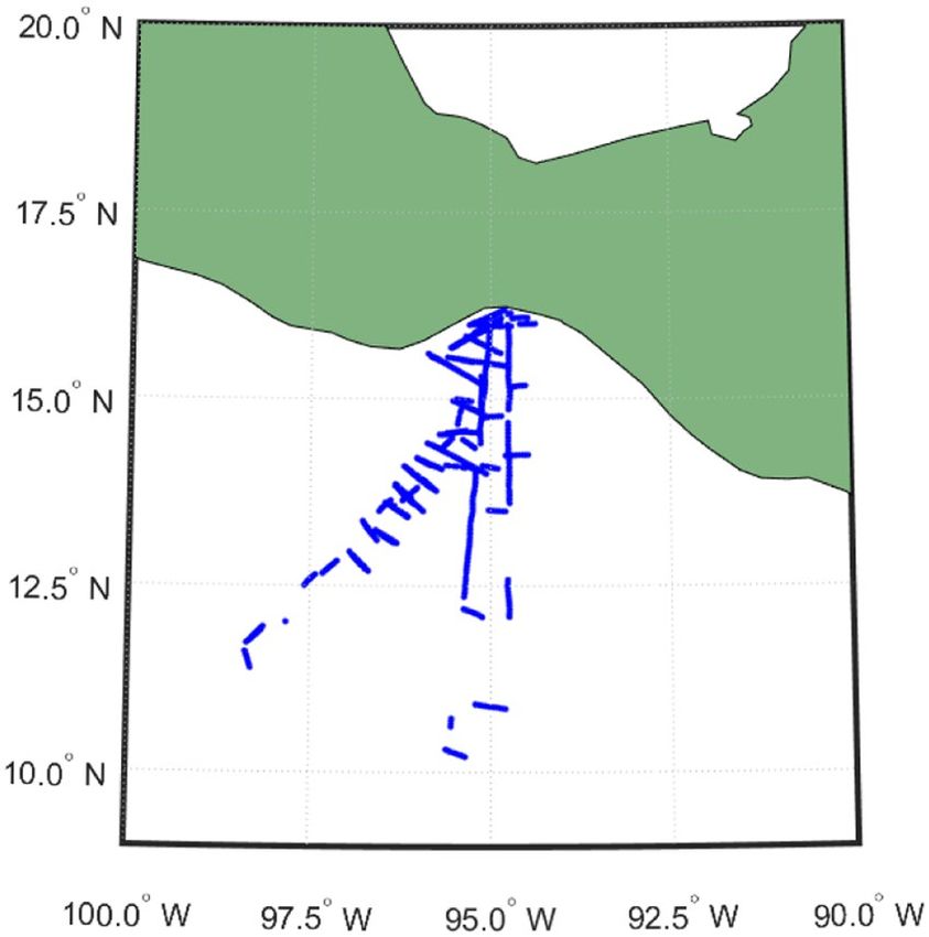
www.nature.com/scientificreports/ www.nature.com/scientificreports
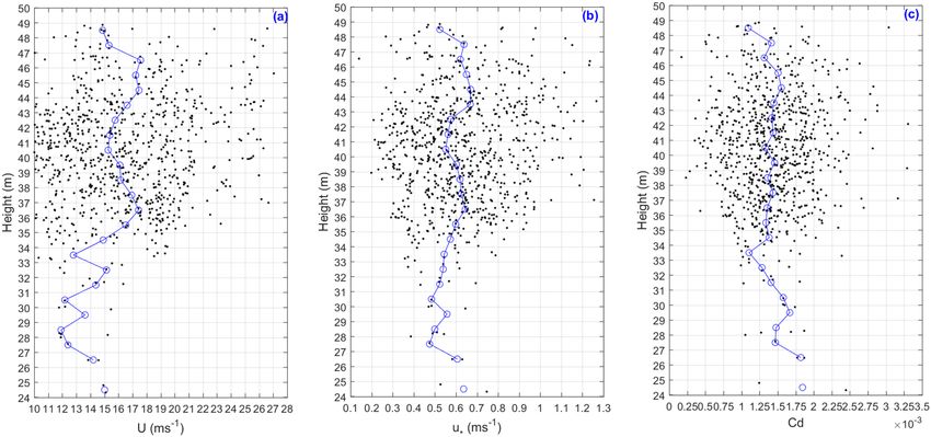
Figure 1. The Geographic locations and flight patterns of the GOTEX experiment.
the magnitude of the drag coefficient became nearly constant at wind speeds above the 23 ms−1 threshold14. This
result is 10–12 ms−1 less than the hurricane-force threshold of 33 ms−1 obtained by the GPS drop sonde meas-
urements10 and the laboratory tank measurements11. Troitskaya et al. calculated theoretically and experimen-
tally the laboratory saturation of the drag coefficient at wind speeds exceeding 25 ms−115. Soloviev et al. verified
the increase of the drag coefficient with wind speed up to 30 ms−1 using the unified wave-form and two-phase
parameterization model16. Golbraikh and Shtemler proposed a semi-empirical model for the estimation of the
foam impact on the variation of the drag coefficient17. They found that the wind speed, at which the fractional
foam coverage is saturated, to be responsible for the difference in the drag coefficient behavior under laboratory
and open-ocean conditions. As Donelan pointed out, previous studies explored the physics behind field or lab-
oratory observations, however, they did not provide a simple prescription that may be used in a fully coupled
(atmosphere-wave-ocean) hurricane prediction model18. Donelan revealed a similar Reynolds number depend-
ence of the oceanic sheltering coefficient, as well as a drag coefficient function of Reynolds number, wave age, and
wind speed18. They showed that the drag coefficient reached its peak at a wind speed of 30 ms−1. However, the
equations derived bring more challenges to modeling efforts, due to its constantly changing parameters that can-
not be measured easily during high wind events18. Green and Zhang proposed an empirical quadratic equation
to parameterize the drag coefficient from the 10-m wind speed19. Peng and Li proposed a parabolic model of the
drag coefficient for storm surge simulations in the South China Sea20. There is a clear lack of agreement on the
parameterization of the sea surface drag coefficient under high wind conditions in the scientific community21,22.
Unlike most of the prior studies, this study is to examine mathematically the dependences of the drag coeffi-
cient on wind speed by using the aircraft data collected during the Gulf of Tehuantepec Experiment (GOTEX) on
the Pacific coast of the Isthmus of Tehuantepec, Mexico, in February 2004. The main objective of this paper is to
develop new parameterization equations of the sea surface drag coefficient (Cd) dependent solely on wind speed.
Materials and Methods
Database. The turbulent fluxes of momentum, heat, and water vapor used in this study were derived from
high-resolution measurements of wind speed, air temperature, and water vapor collected by the National Center
for Atmospheric Research (NCAR) C-130 Hercules aircraft in the Gulf of Tehuantepec Experiment (GOTEX)
on the Pacific coast of the Isthmus of Tehuantepec, Mexico, in February 2004, where not many studies have
been conducted23,24 The geographic locations of the aircraft experiments and points (dots) where the data were
collected on the flight tracks are shown in Fig. 1. The height of the mixed layer was 500 m and the height of the
surface layer was assumed to be around 50–100 m during the experimental period. The wind measurements were
obtained close to the surface (between 25 and 50 m a.s.l.) from the five-hole gust probe system located on the
radome of the aircraft. The fluctuating pressure signals of the five-hole gust probe system were averaged over a
period of 5 seconds to allow for conditions to reach steady-state, so the response time is 5 s. The air temperature
was determined from one of the Rosemount thermometers with response time of 5 s. and the specific humidity
was derived from one of the Lyman-alpha sensors with response time of 0.1 s. Turbulent momentum, heat and
water vapor fluxes were obtained as the covariance of the fluctuations from the mean values, averaged over time
period of 40 s, which correspond roughly to spatial segments of 4 km at the typical aircraft speed. The mean values
were determined over each segment24.
Methods. The sea surface turbulent transfer coefficients for momentum (Cd, usually referred as ‘drag coeffi-
cient’), heat (Ch) and water vapor (Ce) are generally defined as
Scientific Reports | (2020) 10:1805 | https://doi.org/10.1038/s41598-020-58699-9 2
www.nature.com/scientificreports/                                                                   www.nature.com/scientificreports

                           Figure 2. (a) The scattered plot of friction velocity (u*) against wind speed (U) measured during the GOTEX
                           aircraft experiments. The blue line with circle is the median number line and the number of samples for each bin
                           of data was also labeled in blue, and (b) the median values (red dashes) and interquartile ranges (blue boxes) of
                           u* for each bin. The red plus symbols are outliners.

                                                                         u⁎2          (w ′u′)2 + (w ′v ′)2
                                                               Cd ≡              =                         ,
                                                                      u2 + v 2                U2                                             (1)

                                                                                     w ′T ′
                                                                         Ch ≡                   ,
                                                                                 U (T0 − Tair )                                              (2)

                                                                                      w ′q′
                                                                         Ce ≡                   ,
                                                                                 U (q0 − qair )                                              (3)
                                                                                 2            2
                           where u* is the friction velocity, and u⁎ ≡ (w ′u′) + (w ′v ′) ; u and v are the components of horizontal wind
                           speed in the longitude direction and the latitude direction, respectively; w is the vertical wind speed; u', v' and w'
                           are the turbulence fluctuations of u, v and w, respectively; and the overbars indicate the time average; T0 and Tair
                           are the air temperatures at the sea surface and at the measurement height, and T0 is considered to be equal to sea
                           surface temperature; q0 and qair are air specific humidity at the sea surface and at the measurement height, and q0
                           is calculated from the sea surface temperature25.

                                                                               U≡     u2 + v 2 .

                           Results and Discussion
                           The variation of friction velocity (u*) against wind speed (U). Figure 2a shows the scatterplot of fric-
                           tion velocity (u*) against wind speed (U) collected from the GOTEX experiment. Note that we removed data with
                           wind speeds less than 10 ms−1 and use only data collected under high wind conditions as the focus of this study.
                           Overall, u* increased with increasing U. The correlation coefficient between u* and U is 0.88. The low correlation
                           coefficient between u* and U and the discrete distribution of points in Fig. 2a are due to the fact that u* depends
                           not only on U, but also on atmospheric stratification stability and sea surface roughness length, which is related
                           to sea surface state (e.g., wave steepness and wave age)4–6,26. We classed the data into 18 bins of wind speed at an
                           interval of 1 ms−1, and the number of samples for each bin was also labeled in blue in Fig. 2a. The median values
                           (red dashes) and interquartile ranges (blue boxes) of u* for each bin were plotted in Fig. 2b. The red plus symbols
                           are outliners.

                           Parameterization of drag coefficient (Cd). The drag coefficient (Cd) was calculated using Eq. (1).
                           Figure 3a is a scatterplot of drag coefficient (Cd) against wind speed (U), and the median of these observations
                           for each bin is also shown in blue line with circles. Cd increased with increasing U. We tried to use polynomial,
                           exponential, Fourier, Gaussian, and linear functions to regress the relationship between Cd and U. We found that
                           the parabolic relationship obtains the minimum root mean square error (RMSE) and the maximum correlation
                           coefficient, so we regressed the relationship between the drag coefficient Cd and U:

                                                          Cd = − 0.005 × 10⁻³(U − 22.33)2 + 0.0017,                                          (4)

Scientific Reports |   (2020) 10:1805 | https://doi.org/10.1038/s41598-020-58699-9                                                             3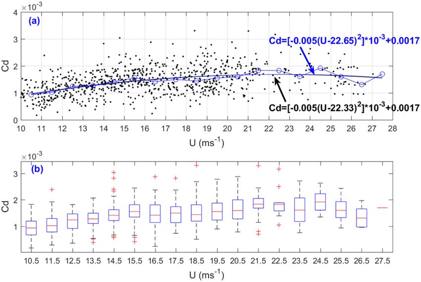
www.nature.com/scientificreports/                                                              www.nature.com/scientificreports

                           Figure 3. Similar to Fig. 2, but for drag coefficient (Cd). (a) the blue line with circle is the median number line.
                           The back line is parabolic regression result for all 806 estimates and the blue line is parabolic regression result
                           for the median number for each bin, and (b) the median values (red dashes) and interquartile ranges (blue
                           boxes) of Cd for each bin. The red plus symbols are outliners.

                           Figure 4. The vertical distribution of (a) wind speed (U), (b) friction velocity (u*), and (c) drag coefficient (Cd).
                           measured during the GOTEX aircraft experiments. The blue line with circle is the median number line.

                              Applying the regression method for the median numbers of bins, we regressed the relationship between the
                           bin median numbers of Cd and U:

                                                          Cd = − 0.005 × 10⁻³(U − 22.65)2 + 0.0017 .                                         (5)
                               We find the parabolic relationships between the drag coefficient Cd and U here. Equations (4) and (5) are very
                           closed to each other. We recommend Eq. (5) because the median method avoids the errors caused by those data
                           points which are too discrete. The “22.65” in Eq. (5) represents the critical (or saturated) wind speed at which Cd
                           reaches its maximum value (0.0017). The result of “22.65” obtained here is lower than results from previous stud-
                           ies9–11. The possible reason is that the wind speeds used in our work are lower than 28 ms−1, and the limited wind
                           speed range brings uncertainty to the regression analysis results. The median values (red dashes) and interquartile
                           ranges (blue boxes) of Cd for each bin were plotted in Fig. 3b. The red plus symbols are outliners.
                               In this study, we calculated the drag coefficient directly from the wind speed measured by aircrafts, and we
                           did not convert the wind speed measured by the aircrafts to the wind speed at a height of 10 meters, since the
                           logarithmic wind profile hypothesis and the constant flux layer hypothesis over the layer may bring additional
                           errors. Recently, by using the data collected during two Floating Instrument Platform field campaigns and the
                           data collected at the Air-Sea Interaction Tower site, Mahrt et al. investigated the relationship between the wind
                           and sea surface stress for contrasting conditions, resulting that the sea surface wind stress decreases significantly

Scientific Reports |   (2020) 10:1805 | https://doi.org/10.1038/s41598-020-58699-9                                                            4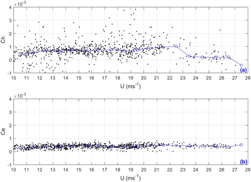
www.nature.com/scientificreports/                                                              www.nature.com/scientificreports

                           Figure 5. Similar to Fig. 3, but for turbulent heat transfer coefficient (Ch) and water vapor transfer coefficient
                           (Ce).

                           Figure 6. (a) The median number variations of drag coefficient (Cd) and enthalpy transfer coefficient Ck
                           against wind speed (U) measured during the GOTEX aircraft experiment; and (b) The value of Ck/Cd against
                           wind speed (U) measured during the GOTEX aircraft experiment.

                           with height near the surface under thin marine boundary layers and/or enhanced stress divergence close to the
                           sea surface conditions27. We plotted variations of U, u* and Cd against height in Fig. 4. It is obvious that the most
                           of data collected at the heights range from 31 m and 49 m. Over all, U increases slightly and u*almost keeps a
                           constant with increasing height, so Cd decrease slightly with increasing height.
                               Equation (5) implies that Cd is negative when U > 41.09 ms−1. Since there is no data higher than 28 ms−1 in
                           our study, we carefully constrain the applicable domain of Eq. (5) to between 10 ms−1 and 28 m−1. Definite con-
                           clusions require more extensive measurements under strong wind conditions.

                           Parameterizations of turbulent heat transfer coefficient (Ch), and turbulent water vapor trans-
                           fer coefficient (Ce). In numerical weather forecasting or climate prediction models, parametric drag coef-
                           ficients, heat transfer coefficients, and water vapor transfer coefficients are usually required at the same time. Do
                           the heat transfer coefficients and water vapor transfer coefficients also have a parabolic increasing behavior with
                           increasing wind speed? Fig. 5 consists two scatterplots of turbulent heat transfer coefficient (Ch) and water vapor
                           transfer coefficient (Ce) with increasing wind speed (U). Figure 5a shows that the distribution of Ch is more
                           scattered than Cd shown in Fig. 3. The reason is that turbulent heat transfer depends not only on the dynamic
                           process but also on the thermal process, and therefore has more complexity and uncertainty. Figure 5 shows that
                           Ch almost remains unchanged when the wind speed is less than 22.65 ms−1, suddenly decreases when U reaches
                           at 22.65 ms−1 and remains at lower values when U is higher than 22.65 ms−1. This is because when the wind
                           speed is greater than 22.65 ms−1, the atmospheric temperature measured by the aircraft remains almost constant
                           (22.42 °C). Unlike Fig. 5a,b shows that the distribution of turbulent water vapor transport coefficients (Ce)is rela-
                           tively concentrated. This is because we assumed that the surface water vapor is saturated during the calculation of

Scientific Reports |   (2020) 10:1805 | https://doi.org/10.1038/s41598-020-58699-9                                                              5
www.nature.com/scientificreports/ www.nature.com/scientificreports
Ce. The median number lines are also plotted on Fig. 5. It is obvious that neither the heat transfer coefficient nor
the water vapor transfer coefficient exhibits a parabolic increase with increasing wind speed.
The maximum storm intensity is sensitive to the ratio of the exchange coefficient of enthalpy (Ck, the exchange
coefficients of heat and water vapor) to the drag coefficient (Cd). We plotted enthalpy transfer coefficient Ck(≡Ch
+ Ce) and Cd in Fig. 6a. Alamaro et al. deduced that the hurricane intensity depends on the value of Ck/Cd9.
Figure 6b shows the variations of Ck/Cd against wind speed. Figure 6b shows that Ck almost remains constant
(0.8) when the wind speed is less than 22.65 ms−1, suddenly decreases to be 0.4 when U reaches at 22.65 ms−1 and
remain at a lower value (0.4) when U is higher than 22.65 ms−1. In the previous literature, we rarely see changes
in Ch with wind speed under strong wind conditions, and we do not see a sudden drop. the value of Ck/Cd.
decreases at U = 22.65 ms−1, mainly due to the sudden decrease in Ck, especially in Ch.
Conclusions
We have established a parabolic relationship between the drag coefficient and wind speed for the data obtained in
the GOTEX experiments. By the regression of wind speed and drag coefficient, we found that the saturated wind
speed is 22.65 ms−1.
Received: 7 August 2019; Accepted: 2 January 2020;
Published: xx xx xxxx
References
1. Garratt, J. R. Review of drag coefficients over oceans and continents. Mon. Weather Rev. 105(7), 915–929, https://doi.
org/10.1175/1520-0493 (1977).
2. Large, W. G. & Pond, S. Open ocean momentum flux measurements in moderate to strong winds. J. Phys. Oceanogr. 11(3), 324–336,
https://doi.org/10.1175/1520-0485 (1981).
3. Yelland, M. & Taylor, P. K. Wind stress measurements from the open ocean. J. Phys. Oceanogr. 26, 541–558 (1996).
4. Oost, W. A. & Oost, E. M. An alternative approach to the parameterization of the momentum flux over the sea. Boundary Layer
Meteorol. 113, 411–426 (2004).
5. Taylor, P. K. & Yelland, M. J. The dependence of sea surface roughness on the height and steepness of the waves. J. Phys. Oceanogr.
31, 572–590 (2001).
6. Gao, Z., Wang, Q. & Wang, S. An alternative approach to sea surface aerodynamic roughness. J. Geophys. Res. 111, D22108, https://
doi.org/10.1029/2006JD007323 (2006).
7. Gao, Z., Wang, L., Bi, X., Song, Q. & Gao, Y. A Simple Extension of “An alternative approach to sea surface aerodynamic roughness”
by Zhiqiu Gao, Qing Wang, and Shouping Wang. J. Geophys. Res. 117, D117, D16110, https://doi.org/10.1029/2012JD017478 (2012).
8. Liu, B., Guan, C. & Xie, L. The wave state and sea spray related parameterization of wind stress applicable from low to extreme winds.
J. Geophys. Res. 117, C00J22, https://doi.org/10.1029/2011JC007786 (2012).
9. Alamaro, M., Emanuel, K. A., Colton, K. A., McGillis, W. R. & Edson, J. Experimental investigation of air-sea transfer of momentum
and enthalpy at high wind speed, paper presented at 25th Conference on hurricanes and Tropical Meteorology, Am. Meteorol. Soc.,
San Diego, Calif., 29 Apr to 3 May (2002).
10. Powell, M. D., Vickery, P. J. & Reinhold, T. A. Reduced drag coefficient for high wind speeds in tropical cyclones. Nature 422(6929),
279–283, https://doi.org/10.1038/nature01481 (2003).
11. Donelan, M. A. et al. On the limiting aerodynamic roughness of the ocean in very strong winds. Geophys. Res. Lett. 31, L18306,
https://doi.org/10.1029/2004GL019460 (2004).
12. Makin, V. K. A note on drag of the sea surface at Hurricane winds. Boundary Layer Meteorology 115(1), 169–176, https://doi.
org/10.1007/s10546-004-3647-x (2005).
13. Kudryavtsev, V. N. & Makin, V. K. Aerodynamic roughness of the sea surface at high winds. Boundary Layer Meteorology 125,
289–303, https://doi.org/10.1007/s10546-007-9184-7 (2007).
14. Black, P. G. et al. Air sea exchange in Hurricanes: Synthesis of observations from the Coupled Boundary Layer Air-Sea Transfer
Experiment. Bull. Am. Meteorol. Soc. 88(3), 357–374, https://doi.org/10.1175/BAMS-88-3-357 (2007).
15. Troitskaya, Y. I. et al. Laboratory and theoretical modeling of air-sea momentum transfer under severe wind conditions. Journal of
Geophysical Research 117, C00J21, https://doi.org/10.1029/2011JC007778 (2012).
16. Soloviev, A. V., Lukas, R., Donelan, M. A., Haus, B. K. & Ginis, I. The air-sea interface and surface stress under tropical cyclones. Sci.
Rep. 4, https://doi.org/10.1038/srep05306 (2014).
17. Golbraikh, E. & Shtemler, Y. M. Foam input into the drag coefficient in Hurricane conditions. Dynamics of Atmospheres and Oceans
73, 1–9 (2016).
18. Donelan, M. A. On the decrease of the oceanic drag coefficient in high winds. Journal of Geophysical Research: Oceans 123,
1485–1501, https://doi.org/10.1002/2017JC013394 (2018).
19. Green, B. W. & Zhang, F. Impacts of air-sea flux parameterizations on the intensity and structure of tropical cyclones. Mon. Wea. Rev.
141, 2308–2324, https://doi.org/10.1175/MWR-D-12-00274.1 (2013).
20. Peng, S. & Li, Y. A parabolic model of drag coefficient for storm surge simulation in the South China Sea. Sci. Rep. 5, 15496, https://
doi.org/10.1038/srep15496 (2015).
21. Anctil, F. & Donelan, M. A. Air water momentum flux observations over shoaling waves. J. Phys. Oceanogr. 2(7), 1344–1352 (2010).
22. Zachry, B. C., Schroeder, J. L., Kennedy, A. B. & Hope, M. E. A case study of near shore drag coefficient behavior during Hurricane
Ike (2008). Journal of Applied Meteorology and Climatology 52(9), 2139–2146, https://doi.org/10.1175/JAMC-D-12-0321.1 (2013).
23. Raga, G. & Abarca, S. On the parameterization of turbulent fluxes over the tropical eastern Pacific. Amer. Chem. Phys. 7, 635–643
(2007).
24. Vickers, D., Mahrt, L. & Andreas, E. L. Estimates of the 10-m neutral sea surface drag coefficient from aircraft eddy-covariance
measurements. J. Phys. Oceanogr. 43, 301–310 (2013).
25. Fairall, C. W., Bradley, E. F., Rogers, D. P., Edson, J. B. & Young, G. S. Bulk parameterization of air-sea fluxes for TOGA COARE. J.
Geophys. Res. 101, 3747–3764 (1996).
26. Oost, W. A., Komen, G. J., Jacobs, C. M. J. & van Oort, C. New evidence for a relation between wind stress and wave age from
measurements during ASGAMAGE. Boundary Layer Meteorol. 103, 409–438 (2002).
27. Larry, M., Scott, M., Tihomir, H. & James, E. On Estimating the Surface Wind Stress over the Sea. Journal of Physical Oceanography
48(7), 1533–1541, https://doi.org/10.1175/JPO-D-17-0267.1 (2018).
Scientific Reports | (2020) 10:1805 | https://doi.org/10.1038/s41598-020-58699-9 6www.nature.com/scientificreports/ www.nature.com/scientificreports
Acknowledgements
This study was supported by the National Key Research and Development Program of Ministry of Science
and Technology of China (2018YFC1506405), and by National Natural Science Foundation of China (Grants
41275022, 41675009 and 4167018). This paper was guided by Professor Larry Mahrt (Northwest Research
Associates) and his very helpful comments are gratefully acknowledged. We thank all dedicated scientists who
collected and made available the fast response aircraft data. The database used in this work was created by the
North West Research Associates under the U.S. Office of Naval Research (ONR) supports. We are very grateful to
two anonymous reviewers for their careful review and valuable comments, which led to substantial improvement
of the manuscript.
Author contributions
Zhiqiu Gao and Wenwu Peng gathered and processed the measurements, Zhiqiu Gao wrote the original draft,
Chole Y. Gao and Yubin Li revised and edited the manuscript.
Competing interests
The authors declare no competing interests.
Additional information
Correspondence and requests for materials should be addressed to Z.G. or Y.L.
Reprints and permissions information is available at www.nature.com/reprints.
Publisher’s note Springer Nature remains neutral with regard to jurisdictional claims in published maps and
institutional affiliations.
Open Access This article is licensed under a Creative Commons Attribution 4.0 International
License, which permits use, sharing, adaptation, distribution and reproduction in any medium or
format, as long as you give appropriate credit to the original author(s) and the source, provide a link to the Cre-
ative Commons license, and indicate if changes were made. The images or other third party material in this
article are included in the article’s Creative Commons license, unless indicated otherwise in a credit line to the
material. If material is not included in the article’s Creative Commons license and your intended use is not per-
mitted by statutory regulation or exceeds the permitted use, you will need to obtain permission directly from the
copyright holder. To view a copy of this license, visit http://creativecommons.org/licenses/by/4.0/.
© The Author(s) 2020
Scientific Reports | (2020) 10:1805 | https://doi.org/10.1038/s41598-020-58699-9 7You can also read