Dynamics of Structure Formation
←
→
Page content transcription
If your browser does not render page correctly, please read the page content below
Dynamics of Structure Formation

The emergence of structures over a broad range of scales from
a highly homogeneous early Universe is one of the key areas of
study in cosmology. Some simple tools have been developed
to describe the evolution of density perturbations in the linear
regime
Overview
 n    Physics of density perturbation evolution

 n    Dynamics of perturbations in the linear regime

 n    Power Spectra and Transfer functions

 30. Apr 2021            Cosmology and Large Scale Structure - Mohr - Lecture 2   2
Our universe then and now

  Recombination (~400,000 yr)
  dr/ ~ 10-5

Cosmic Background Explorer (NASA)

     Present (~14x109 yr)
     dr/ ~ 106
  30. Apr 2021              Cosmology and Large Scale Structure - Mohr - Lecture 2   3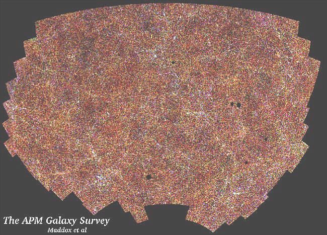
Large Scale
Structure

Harvard-Smithsonian
Center for Astrophysics

                                                           Las Campanas Redshift Survey
 30. Apr 2021             Cosmology and Large Scale Structure - Mohr - Lecture 2          4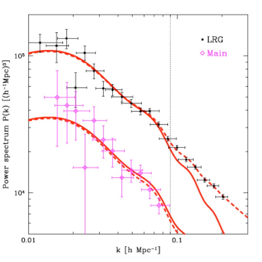
Density perturbations
n Study of the evolution of density perturbations is cast in terms of the evolution
of the dimensionless (energy) density perturbation d
ρ( x )
1+ δ ( x ) ≡
ρ
n Density content is divided into non-relativistic matter and radiation (relativistic
matter)
€
n Adiabatic perturbations: variations in number density that affect all species
by the same factor. Imagine small compressions or expansions. This implies
different energy density variations in the two species
δ r = 43 δ m
n Isocurvature perturbations: “entropy perturbations: where the total density
remains constant, so ρrδ r = −ρmδ m
n At times early compared€
to matter-radiation equality, these perturbations correspond to
variations in the matter density that are offset by miniscule perturbations in the radiation
density
30. Apr 2021 €Cosmology and Large Scale Structure - Mohr - Lecture 2 5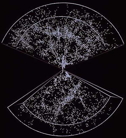
Adiabatic versus Isocurvature
 n    Isocurvature density perturbations seem to be more natural, because
      causality makes it impossible to change density on scales larger than
      the horizon
        n       These perturbations are seeded in late time cosmological phase transition
                models

 n    Within inflationary models the particle horizon is changed at early times
      so that total density fluctuations can be imprinted on scales that appear
      to be larger than the horizon.
        n       If curvature fluctuations are imprinted prior to the process responsible for
                baryon asymmetry then adiabatic modes are norm
                                                                         See discussion in Chapter 11.5, Peacock
        n       Observational evidence of adiabatic density fluctuations then provide good
                support for inflationary models. For example, CMB anisotropy studies allow
                one to constrain the mix of adiabatic and isocurvature fluctuations.
 30. Apr 2021                     Cosmology and Large Scale Structure - Mohr - Lecture 2                           6
Matter and Transfer Functions
n Matter content affects density perturbations through self-gravitation,
pressure and dissipative processes.
n Linear adiabatic perturbations grow as
% a( t ) 2 radiation domination
δ ∝&
' a( t ) matter domination Ω = 1
n Isocurvature perturbations are initially constant and then decline
€ &constant radiation domination
δm ∝ ' −1
( a( t ) matter domination Ω = 1
n In first case, gravity is working to increase the overdensity and in
€
second case gravity is working to maintain the homogeneity.
n In both cases the shape of the density perturbation is unchanged, and
its amplitude is evolving with time
30. Apr 2021 Cosmology and Large Scale Structure - Mohr - Lecture 2 7Pressure Effects: Jeans Instability
n Jeans instability occurs in the collapse of a cloud when the restoring
pressure force is incapable of offsetting the gravitational collapse
during a perturbation
n One can derive the Jeans length by comparing the sound wave
crossing time and the gravitational free fall timescale in a spherical
cloud
n Pressure restoring force unable to react fast enough to stop
gravitational free fall if cloud is too large or too cool
30. Apr 2021 Cosmology and Large Scale Structure - Mohr - Lecture 2 8Jeans length
R
n Consider pressure supported gas
cloud as isolated sphere
%&
n Sound velocity is !"# = %' so for an
,-.
ideal gas we can write !" =
() +=
* /
n Sound wave crossing time:
R π
ts = whereas t ff ≈
cs Gρ
π
n Gravitational free fall timescale λJ = cs
scaling follows from Kepler’s 3rd Gρ 0 > 02 : collapse
law 2 cs3 M> 32 : collapse
4π 3 3
P2 = R M J = 43 πλ ∝
GM J
ρ
3
2 (see next section)
30. Apr 2021 Cosmology and Large Scale Structure - Mohr - Lecture 2 9Pressure Effects in our Universe
n Radiation pressure wins over gravity for wavelengths below the Jeans length
n While the universe is radiation dominated the sound speed is
c
cs =
3
and so the Jeans length
π
λJ = c s
€ Gρ
is always close to the size of the horizon scale.
3 8./
RH = c =c 'ℎ)*) + = 1 ,
H 8π G ρ 3
€
!"
They share same Gr and c scaling and with coefficient above, ratio is #$
~ 8
n Jeans length reaches a maximum at matter-radiation equality and then radiation
becomes tracer population, pressure drops and the Jeans length decreases.
30. Apr 2021 Cosmology and Large Scale Structure - Mohr - Lecture 2 10Comoving Jeans-Length
n The comoving Jeans length at M-R equality is
−1 2 c
Ro rH ( zeq ) = 2 ( )
2 −1 (Ωm zeq )
Ho
≈ 130Mpc
n At larger scales, perturbations should be affected only by gravity, and below this
scale pressure forces are important and growth is slowed or stopped. We will
see that scale is strongly imprinted on the structures in the Universe
n Because this scale depends on the matter density and because the galaxy
distribution reflects the underlying distribution of density perturbations, one
would expect a measure of the galaxy density distribution to provide a
combined constraint on the matter density and the Hubble parameter!
30. Apr 2021 Cosmology and Large Scale Structure - Mohr - Lecture 2 11Small scale effects: Silk damping
n Photon diffusion can erase perturbations in the matter-radiation fluid
n Distance travelled by the photon random walk by the time of the last
scattering is
6 −1 4
λs = 2.7(Ωm ΩB h ) Mpc ≈ 15Mpc
n Within over-density, probability to leave exceeds probability to arrive
n Diffusion of photons out of over-dense regions affects baryons, too,
because the radiation and baryons are tightly coupled prior to
€recombination
n Models with dark matter are less impacted because dark matter
perturbations remain and baryons can fall back into those potential wells
after last scattering
30. Apr 2021 Cosmology and Large Scale Structure - Mohr - Lecture 2 12Small scale effects: Free streaming
n At early times dark matter particles will undergo free streaming at the speed of
light, erasing all scales up to the distance light can travel (horizon)
n This continues until the particles go non-relativistic
c
λ fs =
H(znr )
n For light massive neutrinos (hot dark matter) this happens near zeq, and
essentially all structures on scales smaller than the horizon at M-R equality are
erased. With cold dark € matter the particles are much more massive and go
non-relativistic earlier. These differences lead to dramatically different
structures, and indeed hot dark matter is ruled out.
n A measure of the characteristic amplitude of small scale density fluctuations
prior to their going non-linear should provide a constraint on the dark matter
particle mass (if the dark matter particle is a thermal relic)
30. Apr 2021 Cosmology and Large Scale Structure - Mohr - Lecture 2 13Nonlinear processes
n Most of the directly observable objects in the Universe have
already transitioned well beyond the linear regime, and this
presents a challenge
n Equations of motion can be integrated in N-body simulations, and
extensive work has been done on developing analytical models to
describe nonlinear evolution
n But the distribution of fluctuations in the microwave background,
the clustering of objects on sufficiently large scale, probes of
clustering that extend to the high redshift universe and the number
density of collapsed massive objects like clusters all are examples
of observations whose interpretation relies primarily on linear
evolution of density perturbations
30. Apr 2021 Cosmology and Large Scale Structure - Mohr - Lecture 2 14Overview n Physics of density perturbation evolution n Dynamics of perturbations in the linear regime n Power Spectra and Transfer functions 30. Apr 2021 Cosmology and Large Scale Structure - Mohr - Lecture 2 15
Gravitational dynamics of linear
perturbations
n One can study the evolution of density perturbations in the linear
regime within a Newtonian framework
n Euler Dv ∇p
=− − ∇Φ
dt ρ
n Energy Dρ
= −ρ∇⋅ v
dt
€
n Poisson ∇ 2Φ = 4 πGρ
€
D ∂
n Material or total derivative with convective term = + v⋅ ∇
dt ∂t
€
n Then introduce perturbations as r=ro+dr and v=vo+dv and collect
terms that are first order in the perturbed€quantities. Introduce
δρ
δ≡
ρo
30. Apr 2021 Cosmology and Large Scale Structure - Mohr - Lecture 2 16First order perturbation evolution
n To first order in the perturbed quantities,
the governing equations become:
d ∇δp
δv = − − ∇δΦ − (δv ⋅ ∇)v o
dt ρo
d
δ = −∇⋅ δv
dt
€
∇ 2δΦ = 4 πGρoδ
€
where d/dt is the time derivative of an d ∂
€
observer comoving with the unperturbed = + vo ⋅ ∇
dt ∂t
expansion of the universe
€
30. Apr 2021 Cosmology and Large Scale Structure - Mohr - Lecture 2 17Comoving coordinates
n Through a transformation to comoving coordinates it is possible to
describe the evolution of the perturbed quantities with respect to
overall uniform expansion. We introduce
x (t) = a(t) r (t)
δv (t) = a(t) u(t)
1 ∇δΦ
and use ∇x = ∇r g=
€
a a
˙ a˙ g ∇δp
u+2 u = −
a a ρo
€ €
n The dynamical equations become δ˙ = −∇⋅ u
∇ 2δΦ = 4 πGρoδ
30. Apr 2021 Cosmology and Large Scale Structure - Mohr - Lecture 2 18Differential equation for perturbation
n Using an equation of state 2∂p
definition of the sound speed c ≡s
∂ρ
n And considering a plane wave
−ik ⋅ r
perturbation € δ ∝e
where k is the comoving
wavevector
˙ & 2 2)
we obtain: ˙δ˙ + 2 a δ˙ = δ ( 4 πGρ − c s k +
o 2
a ' a *
€
30. Apr 2021 Cosmology and Large Scale Structure - Mohr - Lecture 2 19
€The non-expanding case
n Without the uniform expansion, the differential equation is
δ˙˙ = δ ( 4 πGρo − c s2 k 2 )
n With solutions of the form
δ (t) = e ±t τ where τ = 1/ 4 πGρo − c s2 k 2
n
€
This solution underscores the possibility of pressure stability
and one can see the critical Jeans length lJ=2p/kJ in the
exponent which governs the transition from real to imaginary t
€ π
λJ = c s
Gρ
30. Apr 2021 Cosmology and Large Scale Structure - Mohr - Lecture 2 20Evolution during radiation domination
n Sound speed differs and the overall treatment we just discussed is
inappropriate 2
2 c
c =
s
3
n The constraint equations become:
Dv D ∂
dt
= −∇Φ
dt
( ρ + p €
c 2
) =
∂t
( p c 2 ) − ( ρ + p c 2 )∇⋅ v ∇ 2Φ = 4 πG( ρ + 3 p c 2 )
€ n The differential
€ equation describing evolution
€ of the overdensity
2
becomes (where we have used p = ρc 3 )
˙δ˙ + 2 a˙ δ˙ = 32π Gρ δ
o
a 3
30. Apr 2021 Cosmology and Large Scale Structure - Mohr - Lecture 2 21Solutions for d(t)
n If we try a power law solution in t we obtain
2
δ (t) ∝ t 3
or t −1 matter dominated
δ (t) ∝ t1 or t −1 radiation dominated
n Remember that for W=1, according to the Friedmann equation, the
scale factor grows as 2
€ a(t) ∝ t 3
matter dominated
1
a(t) ∝ t 2
radiation dominated
Giving us simple solutions for the growth of density perturbations for these
two cases (early and intermediate times)
€ δ∝a matter dominated
δ ∝ a 2 radiation dominated
As dark energy comes to dominate at late times the solution deviates from
these simple cases
30. Apr 2021 Cosmology and Large Scale Structure - Mohr - Lecture 2 22
€What about velocity perturbations?
˙ a˙ g ∇δp
n Where density perturbations are growing there u+2 u = −
has to be inflow of material. a a ρo
δ˙ = −∇⋅ u
∇ 2δΦ = 4 πGρoδ
n Note that the gradient in the peculiar velocity field is related to the growth
rate of the density perturbation €
n Peculiar velocities react to the matter directly- no complicating bias factor
n The derivative introduces different spatial weighting for velocities as
compared to overdensity (see Dodelson 9.2)
ifaH δ ( k, a ) a dD
u ( k, a ) = where f≡ and δ ( k, a ) = δ0 D
k D da
n where f is a dimensionless growth rate.
f ≈ Ω0.6
m
30. Apr 2021 Cosmology and Large Scale Structure - Mohr - Lecture 2 23Overview n Physics of density perturbation evolution n Dynamics of perturbations in the linear regime n Power Spectra and Transfer functions 30. Apr 2021 Cosmology and Large Scale Structure - Mohr - Lecture 2 24
Observed distributions of objects, matter and
temperature constrain density perturbations
                                                                      Las Campanas Redshift Survey
 l(l+1)Cl /2π (μK)2

                      l                                                    CMB Temperature Fluctuations
 30. Apr 2021             Cosmology and Large Scale Structure - Mohr - Lecture 2                          25
Scale Dependent Variance in Gaussian Field
n Imagine a spatial volume or sky n These statistical descriptions
area where each coordinate cell are powerful in a homogeneous
contains a value drawn from a and isotropic Universe like our
Gaussian distribution own.
n Spatial power spectrum P(k) or n Early Universe models of
spherical harmonic power inflation predict the statistical
spectrum Cl encodes Gaussian properties of the density field
variance as a function of rather than a specific realization
inverse scale
30. Apr 2021 Cosmology and Large Scale Structure - Mohr - Lecture 2 26Density Field and Pairs
n The cosmic density field r is typically expressed in dimensionless form d, where
is the mean
ρ density. We can adopt this also for galaxies.
ρ ( x ) −ρ
δ (x) =
ρ
n The correlation function ξ is defined as the overabundance of galaxy-pairs at
separation r relative to a random distribution. Consider two volumes dV1 and
dV2 separated by vector "⃗ and containing a number of galaxies dN1 and dN2,
where #$ = &' #( and &' is the mean number density. Then the number of pairs
is
! 2 !
()
dN pair r = dN1dN 2 = n0 (1+ ξ ( r ))dV1dV2
n The expected number of pairs in two volumes dV1 and dV2 separated by "⃗ can
also be written as the volume average of the following quantity
! ! !
dN pair = n0 (1+ δ ( x))dVx ⋅ n0 (1+ δ ( x + r ))dVx+r
Cosmology and Large Scale Structure - Mohr - Lecture 2 27Correlation Function and Overdensity
n Averaging over the volume we write
! 1 ! ! ! ! ! !
()
dN pair r = ∫ d 3 x n02 (1+ δ ( x) + δ ( x + r ) + δ ( x) ⋅ δ ( x + r ))dV1dV2
V VolumeV
2
⎧⎪ 1 3 ! ! ! ⎫⎪
= n dV1dV2 ⎨1+
0 ∫ d x δ ( x)δ ( x + r )⎬⎪
⎪⎩ V VolumeV ⎭
Because 3 !
n
∫ d x δ ( x) =0
VolumeV
n By comparing this expression with
! !
dN pair r = dN1dN 2 = n02 (1+ ξ ( r ))dV1dV2
()
we see that: ξ ( r ) = δ ( x)δ ( x + r )
The (auto)correlation function is just the expectation value of the product of the
overdensity field times the field offset by vector "⃗
Cosmology and Large Scale Structure - Mohr - Lecture 2 28Correlation Function and Power Spectrum
n The correlation function is the convolution of the overdensity field with itself
(offset by distance r)– so the auto-correlation function
ξ ( r ) = δ ( x)δ ( x + r ) = (δ ⊗ δ )r
n This helpful, because we remember that the convolution theorem states that the
convolution of two quantities can be expressed as the Fourier transform of the
product of the Fourier transforms of each of the quantities.
! ! ! !
ξ ( r ) = δ ( x)δ ( x + r )
V !!
∗ −ik ⋅r 3 3 ! ik!⋅x!
=
(2π )3
∫δ δ e
k k ()
d k where δk = ∫ d x δ x e
V 2 !!
−ik ⋅r
= ∫δ k
e d 3k
(2π )3
where we differentiate between the overdensity field δ #⃗ and its Fourier transform $% &
()
using a subscript k. k is wavenumber with inverse length scaling & = *
Cosmology and Large Scale Structure - Mohr - Lecture 2 29Correlation Function and Power Spectrum
n If we write the power spectrum as P(k)=|dk|2
then the correlation function is the so-called Fourier transform pair of the power
spectrum
1 ikr 3 V −ikr 3
P (k ) =
V
∫ ( ) d r and ξ (r ) =
ξ r e 3 ∫ ( ) dk
P k e
( 2π )
Further, because the Universe is isotropic, we have dropped the vector
quantities "⃗ and # and use only their amplitudes r and k
n We will see that from the theory side the power spectrum is of particular
use, while on the observational side both power spectrum and
correlation functions are used to characterize the data
Cosmology and Large Scale Structure - Mohr - Lecture 2 30Power Spectrum ! 1 ! ik⋅! r!
n Fourier analyses are particularly convenient
() V
3
δ k = ∫ d r δ (r ) e
for many applications ! V ! −ik⋅! r!
δ #⃗ and $% & are Fourier transform pairs δ (r ) =
( 2π )
3 ∫
3
d kδ k e ()
The power spectrum encodes the second 1
n
moment of the overdensity field (variance, (
P k1, k2 = ) ( 2π )
3 ( )( )
δ k1 δ k2
because zero mean). Statistical
homogeneity and isotropy implies P(k)
contains complete statistical description ( ) (
P k1, k2 = δD k1 − k2 P k1 ) ( )
n Dimensionless form of power spectrum
3
commonly used. k
Encodes probability of density fluctuation existing above Δ 2 (k ) = 2
P (k )
some threshold p(d>dc) as function of k per unit 2π
logarithmic interval dln(k), which is dk/k
30. Apr 2021 Cosmology and Large Scale Structure - Mohr - Lecture 2 31Statistical Description of Density
Perturbations
n A reasonable starting assumption would be a density field where
the phases of different Fourier modes are uncorrelated and
random—say a Gaussian random field
n Within this context the Power Spectrum, which gives the
characteristic variance of these fluctuations as a function of inverse
scale k, contains all the information
2
P(k) ≡ δ k
large k corresponds to short lengths, small k to long lengths
n Gaussianity to a high level is expected from Inflation, and it can be
measured in€the CMB and in the impact that non-Gaussianity would
have on structure formation. We return to this later.
30. Apr 2021 Cosmology and Large Scale Structure - Mohr - Lecture 2 32LSS Constrains Power Spectrum
= Gaussian random field d(x)
= Linear power spectrum P(k)
Las Campanas Redshift Survey
30. Apr 2021 Cosmology and Large Scale Structure - Mohr - Lecture 2 33Power Spectrum and Transfer function
n Real power spectra result from the processing of initial or primordial power
spectra by the physics we’ve been discussing: self-gravitation, pressure, silk
damping and free streaming.
2 n 2
P(k) ≡ δk = Po k T ( k )
n Because this physics and the primordial power spectrum are a function of
scale– that is, all modes of a particular physical scale are affected similarly– it
is convenient to encapsulate these effects in a so-called transfer function
δ k ( z = 0)
Tk ≡
δ k ( z) D(z)
where in this formulation D(z) is the linear growth factor between redshift z and the
present and k is the comoving wavenumber of the mode. The normalization
redshift is unimportant as long as it refers to a time before any scale of interest has
entered the horizon
€
30. Apr 2021 Cosmology and Large Scale Structure - Mohr - Lecture 2 34from slide 31
3
k
Initial Power Spectrum Δ 2 (k ) =
2π 2
P (k )
n Initial perturbations imprinted
during inflation
n Spectral index determines
variation with k
n
P (k ) ≈ k
n n~1 (just below) theoretically
predicted in inflation models.
CMB anisotropy (WMAP) gives
n=0.968+/-0.012
30. Apr 2021 Cosmology and Large Scale Structure - Mohr - Lecture 2 35Scale Invariant Power Spectrum
n The Harrison-Zeldovich “scale invariant” power spectrum has n=1
Δ2 ( k ) ∝ k 3 P(k) ∝ k n +3
n So in terms of density fluctuations a scale invariant spectrum implies higher
characteristic amplitudes for perturbations on smaller scalesà in other words,
it implies bottom up structure formation
n
€a fluctuation in the gravitational potential,
Consider
∇ 2δΦ = 4 πGρoδ ⇒ δΦk = −4 πGρ oδ k /k 2
which scales as dk/k2
n Thus, the HZ spectrum implies scale independent potential (or curvature)
€
fluctuations
Δ Φ2 ( k ) ∝ k −4 Δδ2 ( k ) ∝ k −1Pδ (k) ∝ k n−1
30. Apr 2021 Cosmology and Large Scale Structure - Mohr - Lecture 2 36Inflationary predictions
n Harrison-Zel’dovich spectrum has a similar amount of power in potential
(curvature) fluctuations within logarithmic intervals on all scales. This means that
potential fluctuations with similar amplitudes are coming through the horizon at all
times
n In inflationary models the amplitude of the potential/curvature fluctuations is
related to the value of the expansion parameter H. The Friedmann equation tells
us that exponential expansion requires constant H during an inflationary period,
and therefore over the period of exponential expansion (inflation) a scale invariant
spectrum of density perturbations would be expected
n Detailed inflationary models predict adiabatic perturbations (potential/curvature
fluctuations) that are close to Harrison-Zeldovich but with slightly higher
gravitational potential fluctuation amplitudes on larger physical scales (tilt; n close
to but < 1). This reflects the tendency for the H parameter to have fallen slightly
during inflation
30. Apr 2021 Cosmology and Large Scale Structure - Mohr - Lecture 2 37Linear growth and additional effects
n Calculation of the transfer functions is a technical challenge because
there is a mixture of matter (dm and baryons) and relativistic particles
(neutrinos, photons)
n These technical difficulties have been overcome in publicly available
codes like CMBfast and CAMB, among others.
n Gruber Cosmology Prize winners 2021: Seljak and Zaldarriaga
n There are multiple ways for the power spectrum today to differ from
that which was laid down at early times (during Inflation):
n Jeans mass effects- pressure as a balancing force to gravity
n Damping effects- overdense regions decay through free streaming or Silk
damping
n As growth proceeds it extends into the non-linear regime and this breaks
the scale independent behavior in the linear regime
30. Apr 2021 Cosmology and Large Scale Structure - Mohr - Lecture 2 38Jeans mass effects
n Prior to M-R equality, perturbations that lie inside the horizon are prevented
from growing by radiation pressure. The horizon scale at M-R equality is
2 −1
deq = 39(Ωh ) Mpc ≈ 320 Mpc
n After zeq, perturbations on all scales grow if collisionless dark matter
dominates; however if baryonic matter dominates then the Jeans length
remains approximately constant and growth suppression is maintained through
recombination
€
n The impact on the transfer function depends on the type of perturbation
30. Apr 2021 Cosmology and Large Scale Structure - Mohr - Lecture 2 39T(k) for adiabatic perturbations
n For larger scale perturbations that don’t enter the horizon until after zeq they
undergo growth 2
δ ∝a λ ∝a
c 8π G
2 8π G
dH = H = ρ= ρo a −4 dH ∝ a 2
H 3 3
n For smaller scale perturbations with wavenumber k that enter the horizon prior
to zeq, they enter into a sort of oscillatory stasis due to pressure effects. This
period of “lost growth” suppresses their growth, and the suppressed growth
effect is larger for the smaller perturbations that enter the horizon earlier
n For adiabatic perturbations this implies:
$&1 (kdeqT(k) for isocurvature perturbations
n For smaller scale perturbations that enter the horizon prior to zeq all the
photons disperse (free stream) and only the matter perturbations remain,
which then basically remain constant until after zeq
n Larger scale perturbations that enter after zeq grow from that point on (don’t
grow while outside horizon because remember these perturbations have zero
associated energy density perturbation)
n So the net effect is a kind of opposite behavior relative to the adiabatic
perturbations. For isocurvature perturbations this implies:
*2# & 2
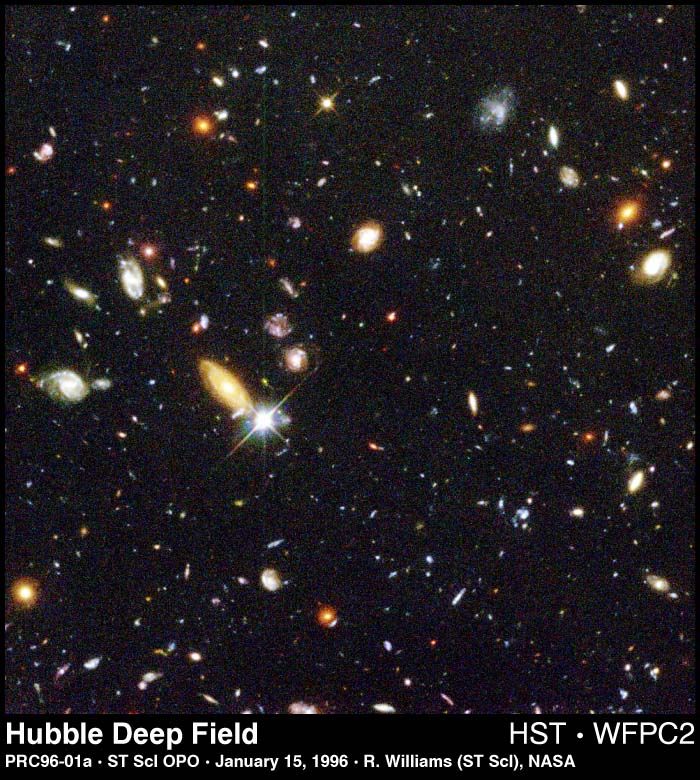
, 15 % kc ( (kdeqTransfer Functions
n This plot from Peacock
illustrates the behavior of
the transfer function in
several cases, including
both adiabatic and
isocurvature as well as
purely CDM, HDM and
baryonic models
2
P(k) ≡ δk = Po k nT 2 ( k )
30. Apr 2021 Cosmology and Large Scale Structure - Mohr - Lecture 2 42Measured Power Spectrum
n In the real Universe one can constrain the power spectrum in a variety of
ways:
n The temperature perturbations of the CMB can be directly connected to the
underlying baryonic density perturbations and underlying matter density
perturbations
n With weak lensing it is possible to constrain the matter density fluctuations more or
less directly
n Often one measures the clustering of objects, whose positions are expected to
reflect statistically the underlying clustering of the matter density field. In a
Gaussian initial density field, objects are expected to exhibit biased clustering with
respect to the underlying DM power spectrum (more on this later). One sees:
2 2 n 2
Pgal (k) = b ( k ) P ( k ) = b ( k ) Po k T ( k ) !"#$ &⃗ ~(!) &⃗
where bias parameter b is expected to be constant on large scales.
30. Apr 2021 Cosmology and Large Scale Structure - Mohr - Lecture 2 43from slide 31
Matter Density Impact on 3
k
Power Spectrum Δ 2 (k ) = 2
P (k )
2π
n During radiation domination dark
matter- radiation coupling leads to
stasis for dark matter density
perturbations on scales below
Jeans scale
n Jeans scale ~ horizon scale
(the largest scale over which supporting
pressure forces can function is the
particle horizon) Low Wm
n Horizon scale at matter-radiation
equality is imprinted on power
spectrum
30. Apr 2021 Cosmology and Large Scale Structure - Mohr - Lecture 2 44Damping effects
n In addition to having growth retarded, small scale perturbations can
actually be erased by damping processes
n For collisionless matter, perturbations are erased by simple free
streaming- random particle velocities lead to net loss from
overdense regions and net gain in underdense regions. At
sufficiently early times the dark matter particles were also relativistic
and could free stream
n Silk damping is important for baryons, because diffusion of photons
out of overdense regions drags the leptons (and their
accompanying baryons) along
30. Apr 2021 Cosmology and Large Scale Structure - Mohr - Lecture 2 45Neutrino Impact on Power Spectrum
n Neutrinos are low mass and
remain relativistic over much of
the history of the Universe
n They free stream out of smaller
scale perturbations, leaving
only dark matter and baryons
behind
n This leads to a reduction of
power on small scales that
increases with the neutrino
fraction
30. Apr 2021 Cosmology and Large Scale Structure - Mohr - Lecture 2 46Baryonic Features in the Power Spectrum
n Baryons are tightly coupled to
the photons until recombination
n Thus, baryon perturbations
have oscillatory solutions
(sound waves)
n Given the ~15% baryon fraction
in the Universe, these features
are observable
30. Apr 2021 Cosmology and Large Scale Structure - Mohr - Lecture 2 47APM Survey Results
n The angular correlation function
analysis was a critical step forward in
testing structure formation models
n It clearly demonstrated inconsistency
between the real universe and the
expectations of the Standard Cold
Dark Matter (sCDM, WM=1) model
which was the theorists favorite at
the time
30. Apr 2021 Cosmology and Large Scale Structure - Mohr - Lecture 2 48Observed Galaxy Power Spectrum
n Observations of the galaxy
power spectrum support
adiabatic density
perturbations.
n CMB anisotropy power
spectrum is also
consistent with
expectations for adiabatic
density perturbations
n Plot from Tegmark page:
http://space.mit.edu/home/te
gmark/sdss.html
30. Apr 2021 Cosmology and Large Scale Structure - Mohr - Lecture 2 49SDSS Correlation Function
n The correlation function of
the SDSS survey is shown
here, and one can see an
interesting feature, which
corresponds to a baryonic
feature at a scale of 150Mpc
that is reflected in the
distribution of galaxies!
n See Eisenstein et al 2005
30. Apr 2021 Cosmology and Large Scale Structure - Mohr - Lecture 2 50Spherical Harmonic Approach
Similarly, one can use the angular power
CMB Temperature Power Spectrum
n
spectrum (Cooray et al 2001) of these tracers 11
SPT + WMAP7
n The angular power spectrum involves
expanding the projected overdensity field in
spherical harmonics
() ()
δ2 θ = ∑ almYlm θ
l,m
n One then examines the equivalent of the 2D
power spectrum, but in this case the treatment
accounts properly for the curved nature of the
sky
2
Cl ≡ alm
Fig. 4.— The SPT bandpowers (blue), WMAP 7 bandpowers (orange), and the lensed theory spectrum for the best-fit ⇤CDM cosmology
n Powerful set of tools available to work with shown for CMB-only (dashed line), and CMB+foregrounds (solid line). As in Figure 3, the bandpower errors shown in this plot do not
include beam or calibration uncertainties.
and the optical depth ⌧ are completely degenerate for Next, we present the constraints on the ⇤CDM
maps- HEALPix http://healpix.jpl.nasa.gov/ the SPT bandpowers, we impose a WMAP 7-based prior
of ⌧ = 0.088 ± 0.015 for the SPT-only constraints.
model from the combination of SPT and WMAP 7 data.
As previously mentioned, we will refer to the joint
We present the constraints on the ⇤CDM model from SPT+WMAP 7 likelihood as the CMB likelihood. We
SPT data and WMAP 7 data in columns two to four of then extend the discussion to include constraints from
Table 3. As shown in Figure 5, the SPT bandpowers CMB data in combination with BAO and/or H0 data.
30. Apr 2021 Cosmology and Large Scale Structure - Mohr
constrain the ⇤CDM -parameters
Lectureapproximately
2
as WMAP 7 alone. The SPT and WMAP 7 parameter
as well
51
We present the CMB constraints on the six ⇤CDM
parameters in the fourth column of Table 3. Adding the
constraints are consistent for all parameters; ✓s changes full survey SPT bandpowers tightens the constraints on
the most significantly among the five free ⇤CDM param- ⌦b h2 , ⌦c h2 , and ⌦⇤ by 33%, 29%, and 31%, respectively,
eters, moving by 1.5 . The constraint on ✓s also tightens relative to WMAP 7. For comparison, the addition ofDirect Measure of Peculiar Velocities
n These peculiar velocities introduce complexities (and opportunities) in the
analysis of clustering within redshift surveys
n The observed redshift includes the “Hubble flow” as well as the component of the
galaxy peculiar velocity along the line of sight.
n In the case where one has an independent measure of the distance, one can
directly measure peculiar velocities
n With a 10% distance measurement one can play this game in the nearby universe
n Expected characteristic peculiar velocity for galaxies is dv~300 km/s, so already at
Hubble flow of 3000km/s (~42Mpc), the effect of the distance uncertainty is
comparable to the scale of the signal one is trying to measure
n This was a driver for 1980’s cosmological studies, using Fundamental Plane
and Tully-Fisher distances
30. Apr 2021 Cosmology and Large Scale Structure - Mohr - Lecture 2 52Power Spectrum Constraints
n Combined constraints on
the power spectrum from
a variety of tracers using
over a range of scales
5x10⁴ in physical scale
and dynamic range in
amplitude of 105
this plot adopts the D2
measure and is plotted
versus scale rather
than wavenumber
n Plot from Tegmark page:
http://space.mit.edu/home/
tegmark/sdss.html
30. Apr 2021 Cosmology and Large Scale Structure - Mohr - Lecture 2 53References
² Cosmological Physics,
John Peacock, Cambridge University Press, 1999
n Cosmological constraints from Galaxy Clustering”
Will Percival (2006)
http://arxiv.org/abs/astro-ph/0601538
30. Apr 2021 Cosmology and Large Scale Structure - Mohr - Lecture 2 54You can also read