Einstein@Home All-sky Search for Continuous Gravitational Waves in LIGO O2 - IOPscience
←
→
Page content transcription
If your browser does not render page correctly, please read the page content below
The Astrophysical Journal, 909:79 (8pp), 2021 March 1 https://doi.org/10.3847/1538-4357/abc7c9
© 2021. The Author(s). Published by the American Astronomical Society.
Einstein@Home All-sky Search for Continuous Gravitational Waves in LIGO O2
Public Data
B. Steltner1,2 , M. A. Papa1,2,3 , H.-B. Eggenstein1,2 , B. Allen1,2,3 , V. Dergachev1,2, R. Prix1,2, B. Machenschalk1,2,
1
S. Walsh1,2,3, S. J. Zhu1,2,4, O. Behnke1,2, and S. Kwang3
Max Planck Institute for Gravitational Physics (Albert Einstein Institute), Callinstrasse 38, D-30167 Hannover, Germany; benjamin.steltner@aei.mpg.de,
maria.alessandra.papa@aei.mpg.de
2
Leibniz Universität Hannover, D-30167 Hannover, Germany
3
University of Wisconsin Milwaukee, 3135 N Maryland Avenue, Milwaukee, WI 53211, USA
4
DESY, D-15738 Zeuthen, Germany
Received 2020 September 25; revised 2020 October 25; accepted 2020 October 28; published 2021 March 8
Abstract
We conduct an all-sky search for continuous gravitational waves in the LIGO O2 data from the Hanford and
Livingston detectors. We search for nearly monochromatic signals with frequency 20.0Hzf585.15 Hz and spin-
down -2.6 ´ 10-9 Hz s-1 f 2.6 ´ 10-10 Hz s−1. We deploy the search on the Einstein@Home volunteer-
computing project and follow-up the waveforms associated with the most significant results with eight further search
stages, reaching the best sensitivity ever achieved by an all-sky survey up to 500 Hz. Six of the inspected waveforms
pass all the stages but they are all associated with hardware injections, which are fake signals simulated at the LIGO
detector for validation purposes. We recover all these fake signals with consistent parameters. No other waveform
survives, so we find no evidence of a continuous gravitational wave signal at the detectability level of our search. We
constrain the h0 amplitude of continuous gravitational waves at the detector as a function of the signal frequency, in
half-Hz bins. The most constraining upper limit at 163.0Hz is h0=1.3×10⁻²⁵, at the 90% confidence level. Our
results exclude neutron stars rotating faster than 5 ms with equatorial ellipticities larger than 10−7 closer than 100 pc.
These are deformations that neutron star crusts could easily support, according to some models.
Unified Astronomy Thesaurus concepts: Gravitational waves (678); Neutron stars (1108); Compact objects (288);
Astronomy data analysis (1858)
Supporting material: tar.gz file
1. Introduction the computing power donated by the volunteers of the
Continuous gravitational waves are expected in a variety of Einstein@Home project.
The results from the Einstein@Home search are further
astrophysical scenarios: from rotating neutrons stars if they
processed using a hierarchy of eight follow-up searches,
present some sort of asymmetry with respect to their rotation
similarly to what was previously done for recent Einstein@-
axis or through the excitation of unstable r-modes (Owen et al.
Home searches (Abbott et al. 2017; Ming et al. 2019; Papa
1998; Lasky 2015); from the fast inspiral of dark-matter objects
et al. 2020).
(Horowitz & Reddy 2019; Horowitz et al. 2020); through
We use LIGO O2 public data (Vallisneri et al. 2015;
superradiant emission of axion-like particles around black
LIGO 2019; Abbott et al. 2021) and, thanks to a much longer
holes (Arvanitaki et al. 2015; Zhu et al. 2020).
coherent-search baseline, achieve a significantly higher sensi-
The expected gravitational wave amplitude at the Earth is
several orders of magnitude smaller than that of signals from tivity than the LIGO Collaboration O2 results in the same
compact binary inspirals, but because the signal is long-lasting frequency range (Abbott et al. 2019; Palomba et al. 2019). Our
one can integrate it over many months and increase the signal- results complement those of the high-frequency Falcon search
to-noise ratio (S/N) very significantly. (Dergachev & Papa 2020a, 2020b), which cover the range from
The most challenging searches for this type of signal are the 500–1700 Hz.
all-sky surveys, where one looks for a signal from a source that The plan of the paper is the following: we introduce the
is not known. The main challenge of these searches is that the signal model and generalities about the search in Sections 2 and
number of waveforms that can be resolved over months of 3, respectively. In Sections 4 and 5 we detail the Einstein@-
observation is very large, and so the sensitivity of the search is Home search and the follow-up searches. Constraints on the
limited by its computational cost. gravitational wave amplitude and on the ellipticity of neutron
In this paper we present the results from an all-sky search stars are obtained in Section 6, and conclusions are drawn in
for continuous gravitational wave signals with frequency Section 7.
f between 20.0 Hz and 585.15 Hz and spin-down -2.6 ´
10-9Hz s-1 f 2.6 ´ 10-10 Hz s−1, carried out thanks to
2. The Signal
Original content from this work may be used under the terms
of the Creative Commons Attribution 4.0 licence. Any further
The search described in this paper targets nearly monochro-
distribution of this work must maintain attribution to the author(s) and the title matic gravitational wave signals of the form described, for
of the work, journal citation and DOI. example, in Section II of Jaranowski et al. (1998). At the output
1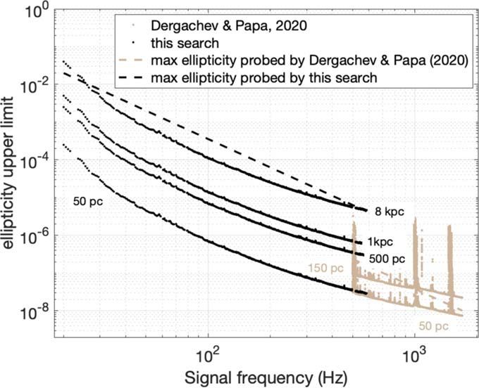
The Astrophysical Journal, 909:79 (8pp), 2021 March 1 Steltner et al.
of a gravitational wave detector the signal has the form
h (t ) = F+ (a , d , y; t ) h+ (t ) + F´ (a , d , y; t ) h´ (t ). (1 )
F+(α, δ, ψ; t) and F×(α, δ, ψ; t) are the detector beam-pattern
functions for the “+” and “×” polarizations, (α, δ) are the R.A.
and decl. of the source, ψ is the polarization angle, and t is the
time at the detector. The waveforms h+(t) and h×(t) take the
form
h+(t ) = A+ cos F (t )
h´(t ) = A´ sin F (t ) , (2 )
with the “+” and “×” amplitudes
1
A+ = h 0 (1 + cos2 i)
2
A´ = h 0 cos i. (3 ) Figure 1. Segmentation of the data used for the Einstein@Home search and the
follow-up stages. The lower two bars show the input SFTs. The first gap in the
The angle between the total angular momentum of the star and data—starting at 70 days—is due to spectral contamination in LHO, based on
the line of sight is 0ιπ and h0 0 is the intrinsic which we decided to exclude this period from the analysis. The second large
gap—starting at ≈120 days—is due to an interruption of the science run for
gravitational wave amplitude. Φ(t) of Equation (2) is the phase detector commissioning.
of the gravitational wave signal at time t. If τSSB is the arrival
time of the wave with phase Φ(t) at the solar system barycenter, likelihood ratio of the data containing Gaussian noise plus a
then Φ(t)=Φ(τSSB(t)). The gravitational wave phase as a signal with the shape given by the template, to the data being
function of τSSB is assumed to be purely Gaussian noise.
F (tSSB) = F0 + 2p [ f (tSSB - t0SSB)+ The -statistic values are summed, one per segment (i ),
and, after dividing by Nseg, this yields our core detection
1 statistic (Pletsch & Allen 2009; Pletsch 2010):
f (tSSB - t0SSB )2 ]. (4 )
2
Nseg
1
We take t0 SSB = 1177858472.0 (TDB in GPS seconds) as a ≔
Nseg
å i. (5 )
reference time. i=1
The is the average of over segments, in general computed
3. Generalities of the Searches
at different templates for every segment. The resulting is an
3.1. The Data approximation to the detection statistic at some template “in-
We use LIGO O2 public data from the Hanford (LHO) and between” the ones used to compute the single-segment i . In
the Livingston (LLO) detectors between GPS time 1167983370 fact these “in-between” templates constitute a finer grid based
(2017 January 9) and 1187731774 (2017 August 25). This data on which the summations of Equation (5) are performed.
has been treated to remove spurious noise due to the LIGO The most significant Einstein@Home results are saved in the
laser beam jitter, calibration lines and the main power lines top list that the volunteer computer (host) returns to the
(Davis et al. 2019). Einstein@Home server. For these results the host also
We additionally remove very loud short-duration glitches recomputes at the exact fine-grid template point. We
(B. Steltner et al. 2021, in preparation) and substitute Gaussian indicate the recomputed statistic with a subscript “r,” as, for
noise at frequency bins affected by line contamination (Covas example, in r .
et al. 2018). This is a procedure common to all Einstein@Home In Gaussian noise Nseg ´ 2 follows a chi-squared
searches and it prevents spectral contamination from spreading distribution with 4Nseg degrees of freedom, c 24Nseg (r 2 ). The
to many nearby signal frequencies. The list of cleaned
noncentrality parameter r 2 µ h 02 Tdata Sh , where Tdata is the
frequency bins can be found in the online tar.gz file.
duration of time for which data is available and Sh is the strain
As is customary, the input to our searches is in the form of
power spectral density of the noise. The expected S/N squared
short time-baseline (30 minutes) Fourier transforms (SFTs).
is equal to ρ2 (Jaranowski et al. 1998). For simplicity, in the
These are grouped in segments of variable duration that
rest of the paper, when we refer to the S/N we mean S/N
correspond to the coherent time baselines of the various
squared.
searches, as shown in Figure 1.
If the noise contains some coherent instrumental or
environmental signal, it is very likely that for some of the
3.2. The Detection Statistics
templates the distribution of will have a nonzero
For each search we partition the data in Nseg segments, with noncentrality parameter, even though there is no astrophysical
each segment spanning a duration Tcoh. The data of both signal. The reason is that in this case the data looks more like a
detectors from each segment i are combined coherently to noise+signal than like pure Gaussian noise.
construct a matched-filter detection statistic, the -statistic It is possible to identify a nonastrophysical signal if it
(Cutler & Schutz 2005). The -statistic depends on the presents features that distinguish it from the astrophysical
template waveform that is being tested for consistency with the signals that the search is targeting, for example, if it is present
data. The -statistic at a given template point is the log- only in one of the two detectors, or if it is present only for part
2
The Astrophysical Journal, 909:79 (8pp), 2021 March 1 Steltner et al.
of the observation time. In the past we have used these
signatures to construct ad hoc vetoes, such as the -stat
consistency veto (Aasi et al. 2013a) and the permanence veto
(Aasi et al. 2013b; Behnke et al. 2015). These vetoes are still
widely used although with different names: the “single
interferometer veto” in Sun et al. (2020) and Jones & Sun
(2020) as well as the “persistency veto” of Abbott et al. (2019)
and Astone et al. (2014).
We incorporated the ideas of the -stat consistency veto and
of the permanence veto in the design of a new detection
statistic, bˆ S GLtL . The new detection statistic is an odds ratio
that tests the signal hypothesis against a noise model, which in
addition to Gaussian noise also includes single-detector
continuous or transient spectral lines (Keitel et al. 2014;
Keitel 2016). The subscript “L” in bˆ S GLtL stands for line, “G”
for Gaussian, and “tL” for transient-line. We use this detection
statistic to rank the Einstein@Home results. In this way we Figure 2. Number of searched templates per 50 mHz band as a function of
limit the number of results that make it in the top list but that frequency. The sky resolution increases with frequency causing the increase in
the number of templates. The number of templates in frequency and spin-down
would later be discarded by the vetoes. This frees up space on is 14,970 and 8855 respectively.
the top list for other, more interesting, results.
3.3. The Search Grids
is established, one can determine the computational cost of the
For a rotating isolated neutron star, the template waveform is search. If that is found to be too high, one must decide whether
defined by the signal frequency, the spin-down, and the source to reduce the Tcoh or to increase the mismatch, and repeat the
sky-position. The range searched in each of these variables is procedure. Ultimately the best operating point is a compromise
gridded in such a way that the fractional loss in S/N, or between computational cost and sensitivity.
mismatch, due to a signal falling in-between grid points is on It turns out that for the first stages of all-sky surveys with
average 0.5.
Tcoh of at least several hours, the optimal grids are typically
The grids in frequency and spin-down are each described by
a single parameter, the grid spacing, which is constant over the ones with spacings ? the ones at which the metric
search range. The sky grid is approximately uniform on the approximation of Equation (7) holds. In particular we find that
celestial sphere orthogonally projected on the ecliptic plane. the metric mismatch overestimates the actual mismatch. This is
The tiling is a hexagonal covering of the unit circle with good because it means that in order to achieve a certain
hexagon edge length d: maximum mismatch level, we need fewer templates than what
the metric predicts. On the other hand it means that we cannot
1 m sky predict the mismatch analytically using Equation (7). Instead
d (m sky) = , (6 )
f ptE we must resort to simulating signals, searching for them with a
given grid and measuring the loss in S/N with respect to a
with τE;0.021 s being half of the light travel-time across the perfectly matched template. And we have to do this many times
Earth and msky a constant that controls the resolution of the sky to probe different signals (l 0 values) and different random
grid. The sky grids are constant over 5 Hz bands and the offsets between the template grid and the signal parameters.
spacings are the ones associated through Equation (6) to the This is the basic reason why in this paper we often refer to
highest frequency in each 5 Hz. The resulting number of Monte Carlo studies. In all these studies the choice of signal
templates used to search 50 mHz bands as a function of parameters l 0 represents our target source population, which
frequency is shown in Figure 2. The grid spacings and msky are we assume to be uniformly distributed in spin frequency,
given in Table 1. log-uniformly distributed in spin-down, with orientation cos ι
uniformly distributed between −1 and 1, polarization angle ψ
3.4. The Monte Carlos and the Assumed Signal Population uniformly distributed in |ψ|π/4 and source position
The loss in S/N m (l 0 ) due to the parameters l of a signal uniformly distributed on the sky (uniform in 0αThe Astrophysical Journal, 909:79 (8pp), 2021 March 1 Steltner et al.
Table 1
Overview of the Searches
rsky
Search Tcoh Nseg δf df msky ⟨μ⟩ Δf Df d (8.0 ´ 10-3) Ra Nin Nout
(10−14
(hr) (μHz) Hz s−1) (μHz) (10−14 Hz s−1)
−3
Stage 0 60 64 3.34 32.747 9 8.0×10 0.5 full range full range all-sky L 7.9×10¹⁷ 350 145
Stage 1 60 64 3.34 20 5.0×10⁻⁴ 0.3 850.0 1.2×10⁻¹⁰ 5.0 0.75 350 145 101 001
Stage 2 126 29 1 2 1.0×10⁻⁵ 0.09 130.0 2.0×10⁻¹¹ 0.75 1.99 101 001 11 915
Stage 3 126 29 0.19 2 1.0×10⁻⁷ 0.002 10.0 2.0×10⁻¹² 0.1 2.2 11 915 6 128
Stage 4 250 14 0.025 2 2.5×10⁻⁸ 0.001 0.4 3.2×10⁻¹³ 0.02 4.3 6 128 33
Stage 5 500 7 0.01 1 1.0×10⁻⁸ 0.001 0.17 1.45×10⁻¹³ 0.008 6.0 33 21
Stage 6 1000 2 0.001 0.1 1.0×10⁻⁹ 0.000 2 0.067 6.4×10⁻¹⁴ 0.003 7 10.0 21 18
Stage 7 1 563 2 0.001 0.1 5.0×10⁻¹⁰ 0.000 1 0.05 8.0×10⁻¹⁴ 0.005 15.0 18 8
Stage 8 ≈5 486 1 0.001 0.1 1.0×10⁻¹⁰ 0.000 7 0.032 5 4.25×10⁻¹⁴ 0.002 5 50.0 8 6
Note. We show the values of the following parameters: the number of segments Nseg and the coherent time baseline of each segment Tcoh; the grid spacings df , df , and
msky; the average mismatch ⟨μ⟩; the parameter space volume searched around each candidate, Df , Df , and rsky expressed in units of the side of the hexagon sky-
grid tile of the Stage 0 search (Equation (6)); the threshold value R a used to veto candidates of Stage a (Equation (8)); the number of templates searched (Nin ) and how
many of those survive and make it to the next stage (Nout). The first search, Stage 0, is the Einstein@Home search, hence the searched volume is the entire parameter
space. The other searches are the follow-up stages.
4. The Einstein@Home Search produce a series of diagnostic plots, that we can
4.1. The Distribution of the Computational Load on conveniently access through a GUI (graphical user
Einstein@Home interface) tool that we have developed for this purpose.
This provides an overview of the result-set in any 50
This search leverages the computing power of the Ein- mHz band.
stein@Homeproject. This is built upon the BOINC (Berkeley 2. Identification of disturbed bands: as done in previous
Open Infrastructure for Network Computing) architecture Einstein@Home searches (Singh et al. 2016; Zhu et al.
(Anderson 2004; Anderson et al. 2006; BOINC 2020): a 2016; Abbott et al. 2017; Ming et al. 2019; Papa et al.
system that uses the idle time on volunteer computers to solve 2020) we identify bands that present very significant
scientific problems that require large amounts of computing deviations of the detection statistics from what we expect
power. from a reasonably clean noise background. Such devia-
The total number of templates that we searched with
tions can arise due to spectral disturbances or to
Einstein@Home is 7.9×10¹⁷. The search is split into work
extremely loud signals. We do not exclude these bands
units (WUs) sized to keep the average Einstein@Home
volunteer computer busy for about 8 CPU hours. A total of 8 from further inspection, but we do flag them as this
million WUs are necessary to cover the entire parameter space, information is necessary when we set upper limits. We
representing of order 10,000 CPU years of computing. mark 273 50-mHz bands as disturbed.
Each WU searches 9.8 × 10¹⁰ templates, and covers 3. Clustering: in this step we identify clusters of candidates
50 mHz, the entire spin-down range and a portion of the sky. that are close enough in parameter space that they are
Out of the detection statistic values computed for the 9.8 × likely due to the same root cause. We associate with each
1010 templates, the WU-search returns to the Einstein@Home cluster the template values of the candidate with the
server only the information of the highest 7500 bˆ S GLtL results. highest bˆ S GLtL r , which we also refer to as cluster seed.
This search ran on Einstein@Home between 2018 April and We use a new clustering method (B. Steltner et al. 2021,
2019 July, with an interruption of 8 months at the request of the in preparation) that identifies regions in frequency-spin-
LIGO/Virgo Collaboration, after the authors left the down-sky-position that harbor an overdensity of candi-
Collaboration. dates—a typical signal signature. This method achieves a
lower false dismissal of signals at a fixed false alarm rate,
with respect to the previous clustering (Singh et al. 2017)
4.2. Postprocessing of the Einstein@Home Search
by tracing the S/N reduction function with no assumption
We refer to a waveform template and the associated search on its profile in parameter space. An occupancy veto is
results as a “candidate.” All in all the Einstein@Home search also applied, requiring at least four candidates to be
returns 6.0×10¹⁰ candidates: the top 7500 candidates per WU associated with a cluster. Most candidates have fewer
× 8 million WUs. This is where the postprocessing begins. than three nearby partners, so this clustering procedure
The postprocessing consists of three steps: greatly reduces the number of candidates, namely from
1. Banding: as described in the previous section, each 6.0×10¹⁰ to 350,145.
volunteer computer searches for signals with frequency 4. Follow-up searches: after the clustering we have 350,145
within a given 50 mHz band, with spin-down between candidates, shown in Figure 3. Of these, 1352 come from
−2.6×10⁻⁹ and 2.6×10⁻¹⁰ Hz s−1 and a portion of bands that have been marked as disturbed. We follow all
the sky. The first step of the postprocessing is to gather of them up as detailed in Section 5. The list of the
together all results that pertain to the same 50 mHz band. disturbed 50 mHz bands is provided in the online tar.
We compute some basic statistics from these results and gz file.
4The Astrophysical Journal, 909:79 (8pp), 2021 March 1 Steltner et al.
Figure 3. Detection statistics values of candidates as a function of frequency. The candidates coming from undisturbed bands are blue circles, those from disturbed
bands are red triangles, and those from hardware injections are green squares. An unconventional vertical scale is used in all plots, which is linear below 10 and log10
elsewhere. Left panels: bˆ S GLtL r and 2r value of the loudest candidate (the candidate with the highest bˆ S GLtL r ) over 50 mHz, the entire sky and the full spin-down
range, out of the Einstein@Home search. The increase in detection statistics with frequency is due to the number of searched templates increasing with frequency, as
shown in Figure 2. The orange gridded area in the lower left panel indicates the 3σ expected range in Gaussian noise. Right panels: detection statistics values of the
350,145 candidates that are followed-up. By comparing the right and left panels one can see how we “dig” below the level of the loudest 50 mHz candidate with our
follow-up stages.
In order to give a sense of the overall set of Einstein@Home
results, in the left panels of Figure 3 we show the detection
statistic value of the most significant result from every 50 mHz
band. The large majority of the results falls within the expected
range for noise-only. Most of the highest detection statistic
values stem from hardware injections or from disturbed bands
and are due to spectral contamination, i.e., signals (as opposed
to noise fluctuations) of nonastrophysical origin.
5. The Follow-up Searches
Each stage takes as input the candidates that have survived
the previous stage. Waveforms around the nominal candidate
parameters are searched, so that if the candidate were due to a
signal it would not be missed in the follow-up. The extent of
the volume to search is based on the results of injection-and- Figure 4. Mismatch distributions for the various follow-up searches based on
recovery Monte Carlo studies and is broad enough to contain 1000 injection-and-recovery Monte Carlos. The search setups are chosen so
the true signal parameters for 99.8% of the signal population. that the S/N of a signal increases from one stage to the next. This is achieved
For this reason we also refer to this volume as the “signal- either by increasing the Tcoh of the search and/or by decreasing the mismatch.
We note that even though the average mismatch of Stage 8 is larger than that of
containment region.”5 The containment region in the sky is a the previous two stages, this does not imply that the expected S/N for a signal
circle in the orthogonally projected ecliptic plane with radius out of Stage 8 is smaller.
rsky.
The search setups for Stages 1-8 are chosen so that the S/N
of a signal would increase from one stage to the next. This is in Stage 8, the expected S/N for a signal out of Stage 8 is larger
achieved in two ways: by increasing the Tcoh of the search and/
than that of the same signal out of Stage 7 or 6. This can be
or by using a finer grid and hence by decreasing the average
seen by comparing the values of R8, R7, and R6, in Table 1 (the
mismatch. The mismatch distributions of the various searches
quantity R a is defined below in Equation (8) and is related to
are shown in Figure 4. We note that even though average
the expected S/N increase at Stage a with respect to Stage 0).
mismatch of Stage 8 is larger than that of the previous two
We cluster the results of each search and consider the most
stages, this does not imply that the expected S/N for a signal
significant cluster. We associate to the cluster the parameters of
out of Stage 8 is smaller. In fact, because of the larger Tcoh used
the member with the highest detection statistic value, and refer
5 to this as the candidate from that follow-up stage.
The Monte Carlos were performed with 1839 signals, of which in Stage 1
the chosen containment region contained 1836. For the other stages all the We veto candidates at stage a whose S/N does not increase
signals were recovered within the chosen containment regions. as expected for signals, with respect to Stage 0. We do this by
5The Astrophysical Journal, 909:79 (8pp), 2021 March 1 Steltner et al.
Figure 6. Smallest gravitational wave amplitude h0 that we can exclude from
the assumed population of signals (see Section 3.4). We compare our results
with the latest literature: the Falcon search (Dergachev & Papa 2020a) and the
LIGO results (Abbott et al. 2019) on the same data. There are multiple curves
associated with the LIGO results because they used different analysis pipelines.
hardware injections. Even though we have followed-up
Figure 5. Distributions of R a of candidates from signal injection-and-recovery
Monte Carlos (solid lines) and from the actual search (shaded areas). The
candidates from these bands, we cannot exclude that a signal
dashed-shaded areas show the R a bins associated with the hardware injections. with strength below the disturbance but above the detection
The dashed vertical lines mark the R a threshold values. The dashed horizontal threshold—and hence above the upper limit—could be hidden
lines mark the one-candidate level in the search results. by the loud disturbance, for example, by being associated with
its large noise cluster. Another reason why we cannot guarantee
setting a threshold on the quantity that our upper limit holds in the presence of a disturbance is the
saturation in the Einstein@Home top list that a loud
Stage a
2 r -4 disturbance produces. This prevents candidates from quieter
Ra = . (8 )
2 r
Stage 0
-4 parameter space regions in that band from being recorded.
Given how loud the hardware injections are, for similar
The threshold is set based on signal injection-and-recovery reasons, we also exclude the 50-mHz bands associated with
Monte Carlos, as shown in Figure 5. The values are given in these. The 50-mHz bands where the upper limits do not hold
Table 1. Because of the large number of candidates in the first are provided in the online tar.gz file.
Upper limits are also not given in some half-Hz bands. This
four follow-up stages, the R a thresholds for a=1L4 are
happens for two reasons: (1) if all 50-mHz bands in a half-Hz
stricter than those used for the last four stages. band are disturbed (2) due to the bin-cleaning procedure. In
All the parameters relative to the searches, as well as the Section 3.1 we explained that we remove contaminated
number of candidates surviving each stage, are shown in frequency bins and substitute them with Gaussian noise. If a
Table 1. signal were present in the cleaned-out bins, it too, would be
Only six candidates are left at the output of Stage 8. They are removed. So in the half-Hz bands affected by cleaning, the
due to fake signals present in the data stream for validation upper limit Monte Carlos include the cleaning step after the
purposes, the so-called hardware injections. In fact there are six signal has been added to the data. In this way the loss in
hardware injections with parameters that fall in our search detection efficiency due to the cleaning procedure is naturally
volume, those with ID 0, 2, 3, 5, 10, 11 (LIGO & Virgo 2018). folded into the upper limit. When a large fraction of the half-Hz
We recover them all with consistent parameters. bins is cleaned out, however, the detection efficiency may not
reach the target 90% level. In this case we do not give an upper
6. Upper Limits limit in the affected band. The list of half-Hz bands for which
Based on our null result we set 90% confidence frequentist we do not give upper limits is given in the online tar.gz file.
upper limits on the gravitational wave amplitude h0 in half-Hz Based on the upper limits, we compute the sensitivity depth
bands. The upper limit value is the smallest signal amplitude of the search Behnke et al. (2015) and find values between
that would have produced a signal above the sensitivity level of (49–56) 1 Hz . This is consistent with, and slightly better
our search for 90% of the signals of our target population (see than, the previous performance of Einstein@Home searches
Section 3.4). We establish the detectability of signals based on (Dreissigacker et al. 2018). We provide the power spectral
injection-and-recovery Monte Carlos. The upper limits are density estimate used to derive the sensitivity depth in the
shown in Figure 6 and provided in machine-readable format in online tar.gz file.
the online tar.gz file. We can express the h0 upper limits as upper limits on the
Our upper limits do not hold in some 50-mHz bands, namely ellipticity ε of a source modeled as a triaxial ellipsoid spinning
those marked as disturbed and those associated with the around a principal moment of inertia axis Iˆ at a distance D
6The Astrophysical Journal, 909:79 (8pp), 2021 March 1 Steltner et al.
than 12 ms, within 100 pc of Earth, with ellipticities in the few
×10−7 range and reach the 1×10⁻⁷ mark for spins of 5 ms.
These results probe a plausible range of pulsar ellipticity values,
well within the boundaries of what the crust of a standard neutron
star could support, around 10−5, according to some models
(Johnson-McDaniel & Owen 2013). It is hard to produce a
definitive estimate of such a quantity and it may be that this
maximum value is significantly lower (Gittins et al. 2020). Since
the closest neutron star is expected to be at about a distance of 10
pc (Dergachev & Papa 2020a), it is likely that there are several
hundreds within 100 pc. On the other hand, recent analyses of the
population of known pulsars suggest that their ellipticity should lie
in the 10−9 decade (Woan et al. 2018; Bhattacharyya 2020),
which we reach only for sources rotating faster than 5 ms and
within 10 pc. When the O3 LIGO data is released, its sensitivity
improvement with respect to the O2 data used here (Buikema
et al. 2020) will allow us to extend the reach of our search and
probe ellipticities in the 10−9 decade, at these higher frequencies.
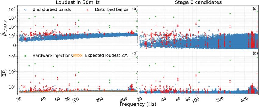
Figure 7. Upper limits on the ellipticity of a source at a certain distance (black). We thank the Einstein@Home volunteers, without whose
We also show the recent upper limits from the low ellipticity all-sky search of
Dergachev & Papa (2020a). The dashed line is the spin-down ellipticity for the support this search could not have happened.
highest spin-down rate probed by each search. We acknowledge the NSF grant No. 1816904.
The follow-up searches were all performed on the ATLAS
(Jaranowski et al. 1998; Gao et al. 2020): cluster at AEI Hannover. We thank Carsten Aulbert and
Henning Fehrmann for their support.
⎛ h0 ⎞ This research has made use of data, software and/or web
e = 1.4 ´ 10-6 ⎜ ⎟
tools obtained from the LIGO Open Science Center (https://
⎝ 1.4 ´ 10-25 ⎠
losc.ligo.org), a service of LIGO Laboratory, the LIGO
⎛ D ⎞ ⎛ 170 Hz ⎞2 ⎛ 10 38 kg m2 ⎞ Scientific Collaboration and the Virgo Collaboration. LIGO is
´⎜ ⎟⎜ ⎟ ⎜ ⎟. (9 )
⎝ 1 kpc ⎠ ⎝ f ⎠ ⎝ I ⎠ funded by the U.S. National Science Foundation. Virgo is
funded by the French Centre National de Recherche Scienti-
The ellipticity ε upper limits are plotted in Figure 7. If the spin- fique (CNRS), the Italian Istituto Nazionale della Fisica
down of the signal were just due to the decreasing spin rate of Nucleare (INFN) and the Dutch Nikhef, with contributions
the neutron star, then our search could not probe ellipticities by Polish and Hungarian institutes.
higher than the spin-down limit ellipticity corresponding to the
highest spin-down rate considered in the search, −2.6×10⁻⁹ ORCID iDs
Hz s−1. This is indicated in Figure 7 by a dashed line. B. Steltner https://orcid.org/0000-0003-1833-5493
Proper motion can reduce the apparent spin-down (Shklovskii M. A. Papa https://orcid.org/0000-0002-1007-5298
1970), so in principle we could detect a signal from a source H.-B. Eggenstein https://orcid.org/0000-0001-5296-7035
with ellipticity above the dashed line. However, even in extreme B. Allen https://orcid.org/0000-0003-4285-6256
cases (source distance 8 kpc, spin period 1 ms, large proper
motion 100 mas yr−1 (Hobbs et al. 2005) or source distance
10 pc, spin period 1 ms and tangential velocity of 1000 km s−1) References
the change in maximum detectable ellipticity is negligible.
Aasi, J., Abadie, J., Abbott, B. P., et al. 2013a, PhRvD, 87, 042001
Aasi, J., Abadie, J., Abbott, B. P., et al. 2013b, PhRvD, 88, 102002
7. Conclusions Abbott, B. P., Abbott, R., Abbott, T. D., et al. 2017, PhRvD, 96, 122004
Abbott, B. P., Abbott, R., Abbott, T. D., et al. 2019, PhRvD, 100, 024004
We present the results from an Einstein@Home search for Abbott, R., Abbott, T. D., Abraham, S., et al. 2021, SoftX, 13, 100658
continuous, nearly monochromatic, gravitational waves with Allen, B. 2019, PhRvD, 100, 124004
frequency between 20.0 and 585.15 Hz, and spin-down Anderson, D. P. 2004, in Proc. 5th IEEE/ACM Int. Workshop on Grid
between −2.6×10⁻⁹ and 2.6×10⁻¹⁰ Hz s−1. We use Computing (Washington, DC: IEEE Computer Society), 4
Anderson, D. P., Christensen, C., & Allen, B. 2006, in Proc. 2006 ACM/IEEE
LIGO O2 public data and compare it against 7.9×10¹⁷ SC06 Conf. (New York: Association for Computing Machinery), 126
waveforms. We follow-up the most likely 350,145 candidates Arvanitaki, A., Baryakhtar, M., & Huang, X. 2015, PhRvD, 91, 084011
through a hierarchy of eight searches, each being more Astone, P., Colla, A., D’Antonio, S., Frasca, S., & Palomba, C. 2014, PhRvD,
sensitive but requiring more per-template computing power 90, 042002
than the previous one. No candidate survives all the stages. Behnke, B., Papa, M. A., & Prix, R. 2015, PhRvD, 91, 064007
Bhattacharyya, S. 2020, MNRAS, 498, 728
This is the most sensitive search performed on this parameter BOINC 2020, http://boinc.berkeley.edu/
space on O2 data, and sets the most stringent upper limits on Buikema, A., Cahillane, C., Mansell, G. L., et al. 2020, PhRvD, 102, 062003
the intrinsic gravitational wave amplitude h0. The most Covas, P. B., Effler, A., Goetz, E., et al. 2018, PhRvD, 97, 082002
constraining h0 upper limit is 1.3×10⁻²⁵ at 163.0 Hz, Cutler, C., & Schutz, B. F. 2005, PhRvD, 72, 063006
Davis, D., Massinger, T., Lundgren, A., et al. 2019, CQGra, 36, 055011
corresponding to a neutron star at, say, 100 pc, having an Dergachev, V., & Papa, M. A. 2020a, PhRvL, 125, 171101
ellipticity of 5×10⁻⁷ and rotating with a spin period of Dergachev, V., & Papa, M. A. 2020b, arXiv:2012.04232
≈12 ms. Our results thus exclude neutron stars rotating faster Dreissigacker, C., Prix, R., & Wette, K. 2018, PhRvD, 98, 084058
7The Astrophysical Journal, 909:79 (8pp), 2021 March 1 Steltner et al.
Gao, Y., Shao, L., Xu, R., et al. 2020, MNRAS, 498, 1826 Palomba, C., D’Antonio, S., Astone, P., et al. 2019, PhRvL, 123, 171101
Gittins, F., Andersson, N., & Jones, D. 2020, arXiv:2009.12794 Papa, M. A., Ming, J., Gotthelf, E. V., et al. 2020, ApJ, 897, 22
Hobbs, G., Lorimer, D., Lyne, A., & Kramer, M. 2005, MNRAS, 360, 974 Pletsch, H. J. 2010, PhRvD, 82, 042002
Horowitz, C., Papa, M., & Reddy, S. 2020, PhLB, 800, 135072 Pletsch, H. J., & Allen, B. 2009, PhRvL, 103, 181102
Horowitz, C. J., & Reddy, S. 2019, PhRvL, 122, 071102 Shklovskii, I. S. 1970, SvA, 13, 562
Jaranowski, P., Krolak, A., & Schutz, B. F. 1998, PhRvD, 58, 063001 Singh, A., Papa, M. A., Eggenstein, H.-B., et al. 2016, PhRvD, 94, 064061
Johnson-McDaniel, N. K., & Owen, B. J. 2013, PhRvD, 88, 044004 Singh, A., Papa, M. A., Eggenstein, H.-B., & Walsh, S. 2017, PhRvD, 96,
Jones, D., & Sun, L. 2020, arXiv:2007.08732 082003
Keitel, D. 2016, PhRvD, 93, 084024 Sun, L., Brito, R., & Isi, M. 2020, PhRvD, 101, 063020
Keitel, D., Prix, R., Papa, M. A., Leaci, P., & Siddiqi, M. 2014, PhRvD, 89, Vallisneri, M., Kanner, J., Williams, R., Weinstein, A., & Stephens, B. 2015,
064023 JPhCS, 610, 012021
Lasky, P. D. 2015, PASA, 32, e034 Woan, G., Pitkin, M., Haskell, B., Jones, D., & Lasky, P. 2018, ApJL,
LIGO 2019, The O2 Data Release, https://www.gw-openscience.org/O2/ 863, L40
LIGO Virgo 2018, https://www.gw-openscience.org/O2_injection_params Zhu, S. J., Baryakhtar, M., Papa, M. A., et al. 2020, PhRvD, 102, 063020
Ming, J., Papa, M. A., Singh, A., et al. 2019, PhRvD, 100, 024063 Zhu, S. J., Papa, M. A., Eggenstein, H.-B., et al. 2016, PhRvD, 94,
Owen, B. J., Lindblom, L., Cutler, C., et al. 1998, PhRvD, 58, 084020 082008
8You can also read