Elsewhere in Australia: a snapshot of temporary mobility on the night of the 2016 Census - UQ eSpace

AUSTRALIAN POPULATION STUDIES                                              2018 | Volume 2 | Issue 1 | pages 14–25

Elsewhere in Australia: a snapshot of
temporary mobility on the night of the
2016 Census
Elin Charles-Edwards* The University of Queensland
Radoslaw Panczak The University of Queensland

* Corresponding author. Email: e.charles-edwards@uq.edu.au. Address: Queensland Centre for
Population Research, School of Earth and Environmental Sciences, The University of Queensland,
Brisbane, Australia 4072
Paper received 13 March 2018; accepted 2 May 2018; published 28 May 2018

Abstract
Background
Temporary population mobility, moves of more than one night’s duration that do not entail a change
in usual residence, are an important feature of the Australian population surface. The ABS Census of
Population and Housing (Census) provides a snapshot of temporary movements one night every five
years.
Aims
This paper examines the intensity, age and spatial patterns of temporary movements captured at the
2016 Census, and creates a classification of regions based on the age profile of movers on Census nights.
Data and methods
2016 Census data were extracted using ABS TableBuilder Pro. Summary metrics were calculated to
measure the intensity and age profile of movements. Origin–destination flows were derived from a
cross-classification of data on Place of Usual Residence and Place of Enumeration. A classification of
regions (SA4s) was constructed from the age profile of movers at origins and at destinations.
Results
1,142,005 individuals (about 5 per cent of the Australian population) were enumerated away from
home on Census night 2016. Mobility peaked in younger (20–30) and older (65–70) age groups. Most
movements were between capital city regions; however, resource regions and coastal areas were
also implicated. The mobility surface was segmented by age: younger people dominated visits to
cities and older movers comprise the majority of visitors to coastal areas, while remote areas had a
significant proportion of visitors in the peak working ages.
Conclusions
Temporary population mobility is selective by age and sex and geographically segmented by these
characteristics. Improved understanding of the attribute of visitors to regions can assist to formulate
and validate estimates of temporary populations from emerging data sets.
Key words
Temporary population mobility; non-residents; spatiotemporal populations; service populations;
migration; Census; Australia.

© Charles-Edwards and Panczak 2018. Published under the Creative Commons Attribution-NonCommercial licence 3.0
Australia (CC BY-NC 3.0 AU). Journal website: www.australianpopulationstudies.org

Australian Population Studies 2 (1) 2018                                 Charles-Edwards E and Panczak R 15

1. Introduction
Temporary population mobility drives significant short-term changes in national population distributions.
Population scholars, particularly in the developed world, have tended to ignore these movements in
favour of permanent migration. This is changing. There is widespread recognition of the implications of
short-term changes in population numbers for service provision (Charles-Edwards and Bell 2013),
emergency response and preparedness (Canterford 2011; Wilson et al. 2016) and disease transmission
(Bharti et al. 2011). Data sets derived from social media (Tenkanen et al. 2017), mobile telephones
(Silm and Ahas 2010; Deville et al. 2014) and other sources are providing new opportunities to monitor
dynamics shifts in population numbers but are not a panacea. They are often partial, suffer from bias
and lack detail on the underlying population flows and the characteristics of movers. It is against this
backdrop that censuses and surveys have continued value for understanding temporary populations.

This short paper explores the intensity and spatial pattern of temporary population mobility, along with
the age and sex of movers, as captured by the Australian Bureau of Statistics (ABS) 2016 Census of
Population and Housing (Census). It provides a short discussion of past studies of temporary population
mobility in Australia in section 2, then in section 3 briefly describes how temporary mobility is captured by
the Census and the limitation inherent in these data. Section 4 reports the intensity of movements and
age profile of movers as captured in 2016, and compares this to data collected at the 1996 Census. In
section 5, the spatial patterns of temporary flows are examined. In section 6, the sex and age characteristics
of movers at origins and destinations are explored. Brief conclusions are presented in section 7.

2. Background
Temporary population mobility can be defined as moves more than one night in duration that do not
entail a change in usual residence (Bell and Ward 2000). This separates temporary mobility from diurnal
movements, such as daily commuting, and from permanent migration. There are some problems with
this definition. Many individuals do not have a single place of usual residence, for example, Fly-in Fly-
out (FIFO)/Drive-In Drive-out (DIDO) miners and children in joint custody arrangements. The distinction
between temporary and permanent mobility may also be unclear, with some ‘temporary’ movements
stretching over years. Notwithstanding, this definition has the advantage of being operationalised using
common Census definitions for Place of Usual Residence and Place of Enumeration.

Temporary population movements are undertaken for a range of reasons. A simple distinction is
between moves undertaken for work or production-related reasons (e.g. FIFO/DIDO mining, seasonal
agricultural labour and business travel) and moves undertaken for consumption-related reasons (e.g.
tourism, second home travel, visits to friends and relatives). Different types of mobility have distinct
spatiotemporal signatures, with diverse destinations, durations, seasonal patterns and periodicities.
For example, FIFO mobility is spatially concentrated in resource regions and follows a common
roster, such as two weeks on site followed by one week at home (McKenzie 2011). By contrast,
coastal tourism can range from a few days to a few weeks in duration, is highly seasonal and
concentrated in the summer months (Charles-Edwards and Bell 2015).

In addition to having distinct spatiotemporal signatures, temporary movers can be segmented
according to age. In a schema proposed by McHugh, Hogan and Happel (1995), mobility in childhood
and adolescence is tied to the family and may include both touristic mobility and mobility associated

16 Charles-Edwards E and Panczak R                                   Australian Population Studies 2 (1) 2018

with family dissolution. In adulthood, mobility becomes increasingly tied to work, which can
necessitate strategies such as long-distance commuting. With the transition to middle age, more
financial resources enable some individuals to purchase second homes, initiating another form of
temporary mobility. Older age may be associated with a relaxation of work-related constraints on
mobility, providing opportunities for new forms of recreational mobility and extended stays with
children and grandchildren, but also additional constraints due to ill health.

There have been a number of studies of temporary population mobility in Australia drawing on
Census data (Bell and Brown 2006), data from the National Visitor Survey (Charles-Edwards, Bell and
Brown 2008) and purposive surveys (Mings 1997; Hanson and Bell 2007). Bell and Ward (1998)
undertook the first systematic study of temporary population mobility in Australia, utilising data from
the 1991 Census. They found that the incidence of temporary mobility remained relatively stable
between the 1976 and 1991 censuses, with around 5 per cent of Australians enumerated away from
home on Census night. The study found that temporary moves tended to cover longer distances than
permanent moves, and revealed a regional pattern of net gains with inner cities, tourist regions and
resource regions all attracting temporary visitors.

Follow up studies comparing temporary and permanent migration (Bell and Ward 2000) and the
characteristics of temporary movers (Bell and Brown 2006) revealed the age profile of temporary
movers, with movements selective of both younger (20–30 years) and older (65–70 years) adults.
Charles-Edwards, Bell and Brown (2008) and Charles-Edwards and Bell (2015), using data from the
National Visitor Survey, confirmed the regionalisation of temporary movements but also the
significant seasonal variation in spatial patterns tied to institutional and climatic factors.

The current study provides an updated account of temporary population mobility in Australia
drawing on data from the 2016 Census. It seeks also to extend our understanding of temporary
moves by examining patterns of origin–destination flows and regional variations in the sex ratio and
age profile of movers. The latter is of particular relevance to agencies interested in providing services
to temporary populations. Data on the age and sex of movers are also critical for the validation of
emerging sources of data on temporary mobility.

3. Data and methods
Data were sourced from the 2016 Census. The Census was conducted on a de facto residence basis,
meaning that people were enumerated where they happened to be on Census night, 9 August 2016. By
combining data on Place of Usual Residence and Place of Enumeration it is possible to generate a snap-
shot of people away from home (referred to as ‘visitors’ through the text) on one night every five years.
The count of the number of people in Australia enumerated away from their Place of Usual Residence
is coded in the Usual Address Indicator (UAICP). UAICP data were extracted from the ABS Counting
Persons, Place of Usual Residence Census database within TableBuilder Pro by age and sex to estimate
the intensity of temporary population mobility on Census night, along with the age profile of movers.

While UAICP provides an estimate of the stock of people enumerated away from home on Census
night, it does not provide information on origin–destination flows. To explore the spatial distribution
of movements, origin–destination matrices were constructed based on individuals’ Place of Usual
Residence (i.e. PUR, the origin) and Place of Enumeration (i.e. POE, the destination) for Statistical

Australian Population Studies 2 (1) 2018                              Charles-Edwards E and Panczak R 17

Areas Level 4 (SA4s). In TableBuilder Pro, PUR data and POE data are only available for cross-
tabulation in the Counting Employed Persons, Place of Work database, which is restricted to
individuals aged 15 years and older. All analyses were done in R (version 3.4.3, R Core Team 2018)
with the circlize package used to draw the flow diagram (Gu et al. 2014). Maps were prepared using
QuantumGIS software (QGIS Development Team 2018).

4. How much movement?
Of 23,401,891 people enumerated on Census night 2016, 1,142,005 (4.9%) were captured away from
their usual residence. In relative terms, this figure has been remarkably stable over the past two
decades, with 4.7 per cent of the population away from home at the 1996 Census (Bell and Ward
2000). When we limit this to adults (aged 15 and over), 5.5 per cent of the population were away from
home. While most moves were over short distances, almost a third of moves were between different
states and territories. In addition to the 4.7 per cent of Australians away from home on Census night,
the Census enumerated 315,530 overseas visitors, equivalent to 1.3 per cent of the 2016 Census count.

Like permanent migration, temporary mobility is highly selective by age and sex. The age schedule of
temporary mobility is bimodal (Figure 1). The highest levels of mobility are among older adults (65–
70 years) and younger adults (20–30 years). The peak in mobility at both older and younger ages
reflects fewer work and family related constraints on these populations on a school night in mid-
winter. The lowest level of mobility is observed among school-aged children, with only 2 per cent
enumerated away from home on Census night. There are marked sex differentials in the mobility age
schedules. Mobility among young women peaks at a younger age and at a lower level than for men.
It then drops to well below the male propensities during key labour force ages before it rises again to
match male levels in retirement.

Figure 1: Per cent of individuals away from home on Census night by age and sex, 1996 and 2016 Censuses
Source: ABS 1996 and 2016 censuses.

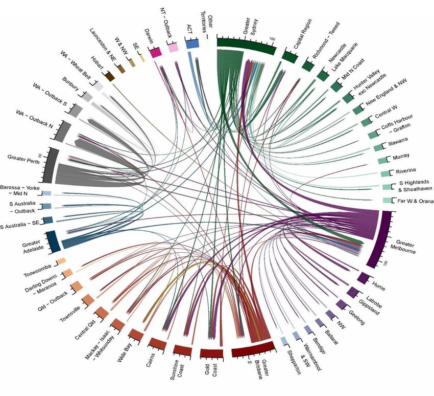
18 Charles-Edwards E and Panczak R                                       Australian Population Studies 2 (1) 2018

How might we explain these differences? The early peak in mobility among females is likely tied to
age differentials in partnering and the absences associated with non-residential relationships. In key
labour force ages, the lower mobility of women might reflect occupational structure, with women
less likely to be employed in roles and industries associated with large amounts of travel (Bell and
Brown 2006). Women are also more likely than men to be constrained by childcaring roles limiting
work-related mobility (ABS 2016). Sex differentials in movement at older ages may again reflect age
differentials in partnering, with a persistent three to four year lag in mobility rates.

There has been an ageing in the profile of movers since the 1996 Census. Mobility has decreased among
younger men, with the percentage away at age 20 declining by more than 25 per cent. This decline has
been offset by a substantial increase in the rate of movement across key labour force ages (25–65). For
women, there has also been a drop in mobility in early adulthood. This is accompanied by a slight increase
in rates between ages 25–45, but also a decline between ages 45–65. Mobility in the retirement ages (65
and over) remained largely unchanged between 1996–2016, while movement intensity in infanthood
dropped for both males and females. Based on the schema set out by McHugh, Hogan and Happel (1995),
these changes suggest a shift away from consumption-related moves, particularly at younger ages,
towards production-related motivations for temporary movements on Census night.

5. Where do people move?

Figure 2: Circular plot showing origin–destination flows between Greater Capital City Statistical Areas and
SA4s (for the rest of Australia), 2016 Census

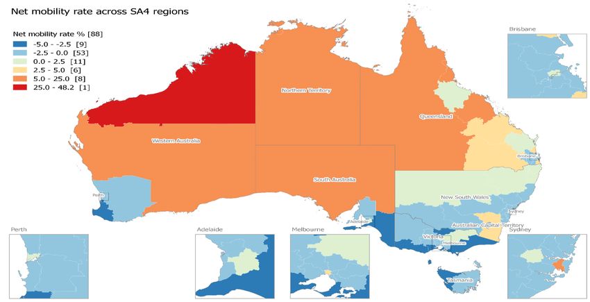
Australian Population Studies 2 (1) 2018                               Charles-Edwards E and Panczak R 19

Figure 2 (above) shows the temporary flows recorded on Census night between Greater Capital City
Statistical Areas (GCCSA) and SA4s (for the rest of Australia). The circular plot represents all inter-SA4
flows, but only shows chords for flows greater or equal to 1,000 people. Colour hues are used to
define Australian states and territories. The direction of the flow is defined by the colour of the origin
and the presence of an arrow at the end of the chord. The width represents the number of movers.

From Figure 2 we learn a number of things. At the national level, we see that the most populous
states of New South Wales, Victoria and Queensland dominate the mobility system in terms of gross
flows (i.e. both ins and outs). The largest flows originate and terminate in metropolitan areas, with
the largest reciprocal flows between Greater Sydney and Greater Melbourne. Greater Brisbane is an
important source of flows to Greater Sydney and Greater Melbourne, but is less attractive as a
destination. Another striking feature is the containment of larger flows within the states and territories,
particularly in the resource states of Western Australia and Queensland. Of all states and territories,
flows from Victoria are the most widely dispersed across Australia, with movers from Victoria recorded
in coastal tourism areas including the Gold Coast, Sunshine Coast and Cairns (all in Queensland).

Figure 3 shows the pattern of net mobility rate (NMR), which captures gains and losses for SA4s.
NMR was calculated by subtracting the number of residents temporarily absent (i.e. out-movers)
from the number of visitors (i.e. in-movers) divided by the usual resident population for each SA4.
The pattern follows a north–south gradient with the greatest gains in northern Australia, including
outback areas of Western Australia, Queensland and the Northern Territory, and the largest losses in
the southern states. Modest gains were also recorded in coastal destinations in southeast
Queensland and northern New South Wales, as well as SA4s encompassing the alpine resort areas of
New South Wales and Victoria. This is consistent with climatic factors dictating the timing and
destination of some forms of temporary mobility (see Charles-Edwards and Bell 2015).

Figure 3: Net mobility rate (%) across SA4s, 2016 Census
Note: Number in brackets indicates number of regions in category.

20 Charles-Edwards E and Panczak R                                               Australian Population Studies 2 (1) 2018

There is also a functional dimension to the mosaic of gains and losses. Capital cities experienced net
population losses except in their urban core, which experienced modest (e.g. Greater Brisbane) to
large (e.g. Greater Sydney) gains. These gains are probably tied to business flows. Gains in northwest
Western Australia and central and southwest Queensland are likely underpinned by mining and oil
and gas extraction-related (FIFO) mobility.

6. Who moves where?
The characteristics of movers are of interest to agencies involved in the planning and provision of
services, as well as to researchers needing denominators for a range of social statistics. Age and sex
are the most critical attributes to be captured.

Figure 4 shows the sex ratio of visitors to SA4s across Australia. The mobility surface is strongly differentiated
by sex. Males dominate temporary moves to resource regions including northwest Western Australia and
central and southern Queensland. The sex ratio is particularly skewed in northwest Western Australia with
more than two male visitors for every female. Sex ratios are also skewed in favour of males in the closely
settled irrigated agricultural zone of southern New South Wales and Victoria. Females dominate visitation
to the suburbs and periphery of most urban areas (except Greater Perth), but not the central business
districts. The sex ratio imbalance is in favour of females in southeast coastal districts of Queensland.

Figure 4: Sex ratio of visitors to SA4s, 2016 Census
Note: The number in brackets indicates the number of regions in each category.

We know that propensity to move varies across the life course. How does this manifest across space?
To explore variations in the age structure of movers in both sending and receiving regions we
grouped SA4s according to the age profiles of individuals temporarily absent from home (represented
as an out-movement rate) and by the age profile of visitors to SA4s (measured as a proportion of all

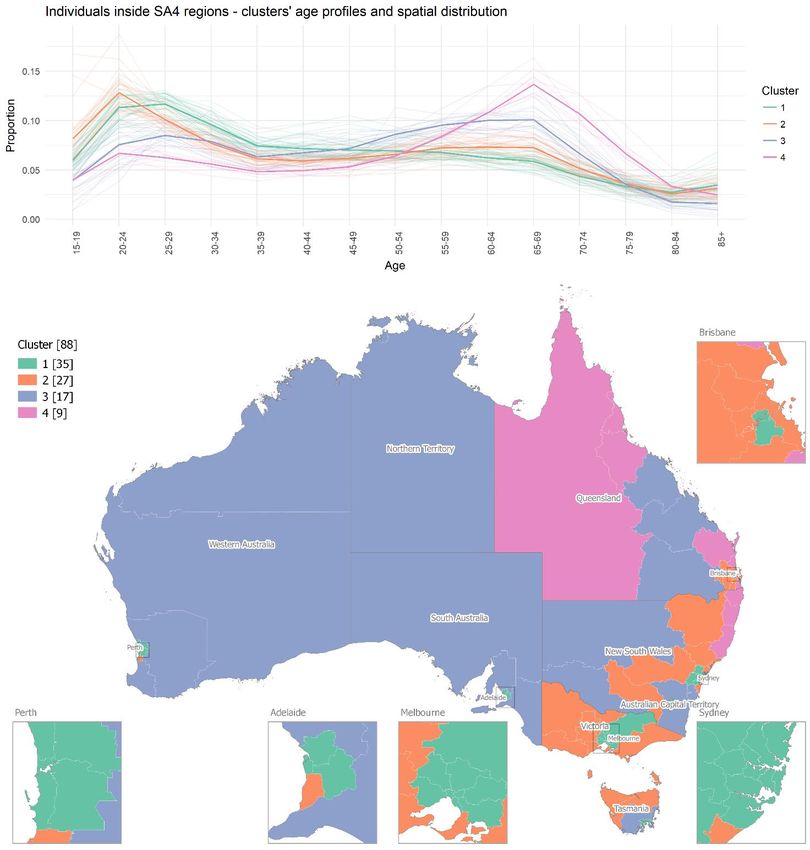
Australian Population Studies 2 (1) 2018                                         Charles-Edwards E and Panczak R 21

visitors to that SA4). Clusters were selected using a k-means clustering algorithm implemented in the
R package stats that determines the optimum partitioning of the dataset for a specified number of
clusters. We derived four groups for residents away from home and four groups for visitors to SA4s.

Figure 5 shows the average age profile of absent residents for each of the four clusters and their
spatial distribution. There are clear differences in both the level and age profile of mobility across
sending regions. Cluster 1 contains the most SA4s (n=28) and comprises the coastal regions of
Queensland and New South Wales, as well as SA4s in Greater Adelaide, Greater Perth, Greater
Darwin and Other Territories (not shown). Outflows from this cluster are of average intensity and
follow a bimodal pattern similar to the national distribution. Sparsely populated outback areas
comprise the majority of SA4s in cluster 2 (n=20). The out-movement rates are the highest (on average)
for younger and middle-aged individuals, and the second highest for individuals aged 65 and over.

Figure 5: Classification of SA4s based on age of absent residents, 2016 Census
Note: The number in brackets indicates the number of regions in each category.

We can surmise that the high level of mobility in part reflects trips to access goods and services
located at considerable distances from home. SA4s in cluster 3 (n=16) have (on average) the highest

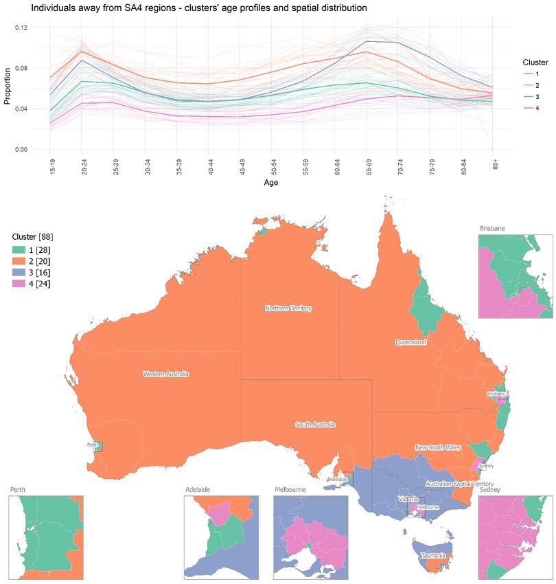
22 Charles-Edwards E and Panczak R                                          Australian Population Studies 2 (1) 2018

proportion of individuals aged 65 and over away from home, and second largest proportion of
people aged 20–29 away from home. SA4s belonging to this cluster are concentrated in the
southeast corner of Australia, which suggests a climatic motivation for absences on Census night.
Cluster 4 is the second largest (n=24) and is characterised by low mobility at all ages. These SA4s are
concentrated in Greater Sydney, Greater Melbourne and Greater Brisbane.

The age profiles of movers are more varied at destinations than at origins. Four clusters are shown in
Figure 6. Note that the clusters are based on the proportion of visitors by age, and thus do not reflect
the level of visitation. The biggest between-cluster differences are at younger ages (below age 35)
and older ages (above age 60). SA4s in cluster 1 (n=35) and cluster 2 (n=27) have younger than
average visitors. Visitors to SA4s in cluster 3 and cluster 4 are older on average.

Figure 6: Classification of SA4s based on age of visitors, 2016 Census
Note: Number in brackets indicates the number of regions in each cluster.

Cluster 1 is comprised of SA4s located in state and territory capital cities. Visitors to these areas are
more likely to be younger or in key labour force ages, suggesting employment as a key driver. Cluster 2
has a similar age profile, but has a higher peak at younger ages and a lower proportion of visitors in

Australian Population Studies 2 (1) 2018                              Charles-Edwards E and Panczak R 23

key labour force ages. SA4s in this cluster are located on the peri-urban fringe of capital cities as well
as southern coastal districts. The cluster includes the southern alpine ski resorts. Cluster 3 (n=18) has
a relatively high proportion of older visitors as well as visitors in key labour force ages. SA4s in this
cluster include the mining resource regions of Western Australia and Queensland, as well as large
swathes of northern Australia which are climatically most attractive during the winter months. This
suggests that a combination of production and consumption motivations are driving visits to these
regions. Visitors to regions in the smallest cluster, cluster 4 (n=9), are older than average with
relatively few individuals below age 50. SA4s belonging to this cluster are located in the coastal areas
of northern New South Wales and southeast Queensland, and in northern Queensland.

7. Discussion and conclusion
Understanding the way in which populations shift over the course of a day, week and month due to
temporary movements is important for planning and service provision, but also for the estimation of
better dominators for a range of health and social statistics. This paper explored the intensity, age
profile and patterns of temporary movements captured at the 2016 Census. It also generated a
classification of regions based on the age profile of residents absent on Census night, and a separate
classification of the age profile of visitors to Australian regions.

The results reveal that the intensity of temporary mobility in Australia has remained stable over the
past two decades, with a rate of around one in twenty. There have, however, been shifts in the age/sex
profile, with movement increasingly dominated by males in key labour force ages. The impact of
temporary population mobility on Census night varies across Australia. Origin–destination flows
connect metropolitan regions, particularly on the eastern seaboard. They distribute people from capital
cities to regions in the resource rich states, and move Victorians to high amenity parts of Queensland.

With respect to impact, the suburbs of major cities and regions in southern Australia experience net
losses. Gains occur in remote and northern Australia, selected high-amenity coastal districts and the
core of major metro regions. When age is taken into account, a more differentiated mobility surface
is revealed. At sending regions there is a close association between accessibility and the level of out-
movement: the more remote an area, the higher the rate of out-movement. At destinations, there is
a bifurcation between regions dominated by younger visitors and those more attractive to older
Australians. The former includes the capital cities and regions in the southeast corner of Australia,
while the latter incorporates the resource regions of central and northern Australia and selected
high-amenity coastal districts.

Census data provides a partial insight into temporary movements in Australia, one night every five
years. It provides no measure of seasonality, duration, frequency or periodicity, nor the complex
circuits and motivations that underpin temporary moves. The spatial patterns observed will not be
replicated at other times of the year: for example, during the January holiday period. The utility of
Census data for the estimation of temporary populations is therefore limited. It does, however, have
the singular advantage of complete enumeration of temporary populations coupled with detailed
information on the characteristics of movers.

The emergence of new data sets, including those collected via social media and communication
technologies, presents further opportunities for the generation of temporary population estimates.

24 Charles-Edwards E and Panczak R                                      Australian Population Studies 2 (1) 2018

However, these data are often partial, biased and confounded by individual behaviour and may not
reliably represent the population present. Baseline data that accurately capture temporary
populations and their characteristics, even if just for a single night, are essential for the production of
robust estimates of non-resident populations. The integration of Census data with emerging data
sets forms a key aspect of an ongoing program of work (the TEMPO project: Techniques for
Estimating Mobile POpulations) aimed at developing techniques for estimating temporary
populations in Australia.

Key messages
•   One in twenty Australians were enumerated away from their Place of Usual Residence on Census
    night 2016. This rate has been stable since 1996; however, the age and sex of movers has
    changed with males in key labour force age groups now much more likely to make temporary
    moves.
•   On Census night temporary flows connect the capital cities in eastern Australia; cities to resource
    regions in Western Australia and Queensland; and Victoria to high amenity parts of Queensland
    and northern and outback Australia.
•   Inner cities and select coastal areas gain temporary movers, while the suburbs and southern
    regions lose residents. This is a winter pattern: the pattern of gains and losses is expected to look
    different in summer months.
•   The age of visitors varies across regions. Understanding these patterns is important for local
    service provision, housing and planning.
•   The complete enumeration of temporary mobility by the Census, even for a single night, provides
    an opportunity to validate estimates of temporary populations derived from new data sources,
    such as social media and mobile phone data.

Acknowledgements
This research was supported through funding from Australian Research Council Linkage Project,
LP160100305, Estimating Temporary Populations (TEMPO project). The authors thank the
anonymous reviewers for their constructive comments that contributed to improving the final
version of the paper.

References
ABS (Australian Bureau of Statistics) (2016) Gender indicators, Australia, Feb 2016. Cat. No. 4125.0.
        Canberra: ABS.
Bell M and Brown D (2006) Who are the visitors? Characteristics of temporary movers in Australia.
        Population, Place and Space 12(2): 77–92.
Bell M and Ward G (1998) Patterns of temporary mobility in Australia: evidence from the 1991 Census.
        Australian Geographical Studies 36(1): 58–81.
Bell M and Ward G (2000) Comparing temporary mobility with permanent migration. Tourism
        Geographies 2(1): 97–107.
Bharti N, Tatem A J, Ferrari M J, Grais R F, Djibo A and Grenfell B T (2011) Explaining seasonal fluctuations
        of measles in Niger using nighttime lights imagery. Science 334(6061): 1424–1427.
Canterford S (2011) Locating people spatially: 2006, 2010, 2100 and 2:36pm on Friday. Australasian
        Journal of Regional Studies 17(1): 46–59.

Australian Population Studies 2 (1) 2018                                 Charles-Edwards E and Panczak R 25

Charles-Edwards E and Bell M (2013) Estimating the service population of a large metropolitan university
        campus. Applied Spatial Analysis and Policy 6(3): 209–228.
Charles-Edwards E and Bell M (2015) Seasonal flux in Australia’s population geography: linking space and
        time. Population, Space and Place 21(2): 103–123.
Charles-Edwards E, Bell M and Brown D (2008) Where people move and when: temporary population
        mobility in Australia. People and Place 16(1): 1–30.
Deville P, Linard C, Martin S, Gilbert M, Stevens F R, Gaughan A E, Blondel, V D and Tatem A J (2014)
         Dynamic population mapping using mobile phone data. Proceedings of the National Academy of
         Sciences 111(45): 15888–15893.
Gu Z, Gu L, Eils R, Schlesner M and Brors B (2014) Circlize implements and enhances circular visualization
        in R. Bioinformatics 30(19): 2811–2812.
Hanson J and Bell M (2007) Harvest trails in Australia: patterns of seasonal migration in the fruit and
       vegetable industry. Journal of Rural Studies 23(1): 101–117.
McHugh K E, Hogan T D and Happel S K (1995) Multiple residence and cyclical migration: a life course
      perspective. Professional Geographer 47(3): 251–267.
McKenzie F H (2011) Fly-in fly-out: the challenges of transient populations in rural landscapes. In: Luck G
       W, Race D and Black R (eds) Demographic Change in Australia’s Rural Landscapes: Implications
       for Society and the Environment. Dordrecht: Springer; 353–374.
Mings R (1997) Tracking snowbirds in Australia: winter sun seekers in far North Queensland. Australian
        Geographical Studies 35(2): 168–182.
QGIS Development Team (2018) QGIS Geographic Information System, Open Source Geospatial
       Foundation http://qgis.osgeo.org.
R Core Team (2018) R: a language and environment for statistical computing. Vienna, Austria,
        R Foundation for Statistical Computing http://www.R-project.org.
Silm S and Ahas R (2010) The seasonal variability of population in Estonian municipalities. Environment
         and Planning A 42(10): 2527–2546.
Tenkanen H , Minin E D, Heikinheimo V, Hausmann A, Herbst M, Kajala L and Toivonen T (2017)
       Instagram, Flickr, or Twitter: assessing the usability of social media data for visitor monitoring in
       protected areas. Scientific Reports 7: article no. 17615. doi: 10.1038/s41598-017-18007-4.
Wilson R, zu Erbach-Schoenberg E, Albert M, Power D, Tudge S, Gonzalez M, Guthrie S, Chamberlain H,
        Brooks C, Hughes C, Pitonakova L, Buckee C, Lu X, Wetter E, Tatem A J and Bengtsson L (2016)
        Rapid and near real-time assessments of population displacement using mobile phone data
        following disasters: the 2015 Nepal earthquake. PLOS Currents Disasters Feb 24. Edition 1. doi:
        10.1371/currents.dis.d073fbece328e4c39087bc086d694b5c.