Evaluating the Reliability of Randomly Acquired Characteristics (RACs) Identification in Footwear Impression Evidence - Corey Katz, Naomi ...
←
→
Page content transcription
If your browser does not render page correctly, please read the page content below
Evaluating the Reliability of Randomly
Acquired Characteristics (RACs) Identification
      in Footwear Impression Evidence
        Corey Katz, Naomi Kaplan-Damary, Hal Stern
                   University of California, Irvine
                         December 2020
                      Email: ckatz@uci.edu
Introduction
• In this presentation, we will discuss a statistical
framework to measure the performance of
footwear examiners, with a focus on randomly
acquired characteristics (RACs) identification.
2Outline of Presentation
• Motivation and Data
• The STAPLE Algorithm
• Hierarchical Framework
• Ongoing/Future Work
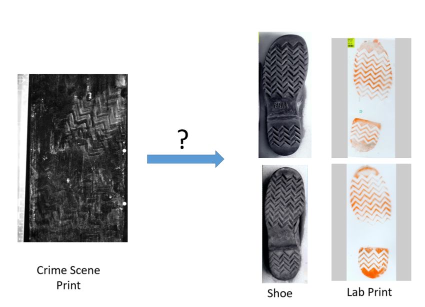
3Shoe Print Evidence
• Shoe prints may be found at crime
scenes and later a suspect's
"matching" shoe is found.
• In court, people are interested if
the suspect's shoe is the source
of the shoe print.
• It can be difficult to identify the
source of the shoe print.
4Shoe Print Examination Process
Step 1:
Rule out any shoes that do not match the basic characteristics of the
suspect shoe (size or tread pattern)
Step 2:
Examine Randomly Acquired Characteristics
Step 3:
Assess the strength of the evidence regarding the hypothesis that
the suspect shoe left the print at the crime scene.
5What is a RAC?
• A randomly acquired characteristic is a unique marking, such as a
scratch or hole, that forms on the sole of footwear as it is being worn.
• Manufacture defects are not considered RACs.
• RACs are examined in order to better assess the evidence regarding
whether or not the suspect shoe left the print at the crime scene.
Examples:
6RAC Identification Challenges
1. Examiners need the physical shoe to find RACs on the lab print.
• Without the physical shoe, differentiating between RACs and
shoe pattern could be difficult
2. Some examiners identify RACs that were not identified by other
examiners.
3. RACs can change overtime
4. Not all RACs appear on both the crime scene print and the
suspects shoe.
• Some are too small to leave an impression or only a partial
print is found.
7Motivation for Understanding the
Reliability of RAC Identification
•Forensic evidence, in general, requires a strong scientific
foundation to be a trusted source of evidence in investigation and
legal proceedings (NRC 2009, PCAST 2016)
• Research on examiner reliability and performance is mainly
focused on the examiner’s ability to match the suspected shoe
print to the source (the final decision) and not on RAC
identification (Hammer et al. 2013, Richetelli et al. 2020).
•Given the importance of RACs in this process, it is important to
explore the reliability of examiners on this task.
8Data 9
Shoe Prints - Our Data

          10
Data
• Data was taken from a pilot study conducted by
CSAFE and the Israel National Police Division of
Identification and Forensic Science.
• 20 shoes (10 Pairs), all of the same brand and
model, worn by police officers.
• Marked by 4 different students that received
some training.
11Data
• This data is valuable because it includes:
• Repeated examinations (same examiner examining
the same impression twice).
• Reproduced examinations (different examiners
examine the same impressions).
• Examinations of the same shoes with different
amounts of wear (45 days, 90 Days, 135 Days,
and180 Days of wear).
• But the data is limited, there are only a few examinations
of each of the above types.
12Variables for Each RAC
• Location on normalized
shoe print (x and y
coordinate of the center of
gravity in 2D space)
• Type of RAC (7 categories)
• Estimated Area of RAC (in
pixels)
• Orientation Angle of RAC
13The STAPLE Algorithm
14Simultaneous Truth And
Performance Level Estimation
• The STAPLE algorithm (Warfield et al. 2004) is an
Expectation-Maximization (EM) algorithm for estimating
the unknown ground truth and examiner performance
parameters in image analysis.
•Developed for brain imaging.
•Relies on having the same image examined by multiple
examiners.
15Data Preprocessing
•In order to implement the STAPLE algorithm, the
data is transformed into binary data.
•This is done by placing a grid over the shoe and
using the location of the RACs to determine
presence/absence of a RAC in each grid cell.
1617
Empirical RAC Prevalence By Examiner
                Shoe\Examiner           A            B            C             D   Naive Estimate*
                  1L45                 NA          0.056        0.055       0.025       0.110
                  1R45                 NA          0.034        0.036       0.042       0.075
                  2L45                0.014        0.017         NA          NA         0.028
                  2R45                0.009        0.008         NA          NA         0.015
                  3L45                0.039        0.034        0.026       0.064       0.103
                  3R45                0.037        0.038        0.038       0.078       0.118
                  4L45                 NA          0.028        0.022        NA         0.043
                  4R45                 NA          0.009        0.010        NA         0.017
                  5L45                 NA          0.026        0.013       0.028       0.053
                  5R45                 NA          0.003        0.010       0.020       0.033
                  7L45                0.015        0.018        0.028       0.020       0.064
                  7R45                0.027        0.014        0.029       0.019       0.064
                  9R45                 NA          0.012         NA         0.014       0.024
                  10L45                NA          0.026        0.024       0.042       0.077
                  10R45                NA          0.010        0.008       0.022       0.037

* All cells with a RAC by any examiner divided by the number of cells (1200).
Notation
N: number of cells in the grid (n × m)
J: number of examiners
Dij: binary presence/absence of RACs in cell i (i = 1 : N) as determined by locations marked by examiner j ( j = 1 : J)
D : the N × J matrix of observed data
Ground Truth Parameters:
Ti: true binary presence/absence of RACs in cell i (i = 1 : N)
T : The length N vector of true presence/absence of RACs
π: Prevalence of RACs on the Shoe
Performance Parameters:
pj: Sensitivity of examiner j
qj: Specificity of examiner j
p ,⃗ q :⃗ J length vectors of sensitivity and specificity
19Model
Complete Data: (D, T)
Observed Data: (D)
Ti ∼ Bernoulli(π)
pj = P(Dij = 1 | Ti = 1).
qj = P(Dij = 0 | Ti = 0).
ti (1−ti)
(Observed Data) Dij | Ti = ti, pj, qj ∼ Bernoulli(pj (1 − qj) ).
An EM algorithm is used to find the maximum likelihood estimates of the parameters.
20Example - Shoe 3L45
Lower Bound Upper Bound
Estimates
95% CI 95% CI
π 0.0574 0.0344 0.0804
pA 0.5438 0.3705 0.7172
pB 0.5010 0.3389 0.6810
pC 0.3312 0.1900 0.4724
pD 0.5829 0.4107 0.7552
qA 0.9916 0.9833 0.9998
qB 0.9948 0.9878 1.0000
qC 0.9928 0.9867 0.9989
qD 0.9674 0.9551 0.9797
21Limitations of STAPLE
•Analyzes each shoe separately.
•Examiners can appear to perform well on some shoes and poorly on
others.
•Performance on one shoe should be related to performance on others.
•Makes strong assumptions about the relationship between the
cells on the grid (independence).
•Only incorporating location information (not type, size of RAC).
22Multi-Shoe Extension
• We incorporate information from images of multiple
shoes at the same time. This is accomplished by
following the same process as outlined above with
theses changes:
1. We assume shoes are independent.
2. This allows us to “average” over the shoes.
Note: Not every examiner has to examine every shoe.
23Results: Multi-Shoe Extension
24Limitations of this Extension
•Each examiner has a single specificity and sensitivity
that applies to all shoes but we know that there is
variation in the difficulty associated with impressions.
• The examiners have similar training, so it may make
sense to model the performance parameters of
examiners jointly.
25Hierarchical Framework
The following model is analogous to STAPLE with the addition of a population structure on the
performance parameters:
μp , νp μq , νq π1 ... πK
... ... ... ...
p1, . . . , pJ q1, . . . , qJ T1,1, . . . , TN,1 T1,K, . . . , TN,K
∀i, j, k
Di,j,k
26Ongoing/Future Work
1. Fully Bayesian analysis of the hierarchical STAPLE
algorithm.
• Provides the necessary framework to expand
model and understand population performance.
2. Autoregressive Model for RAC locations (Spatial
Dependence).
3. Clustering Examiners based on performance.
27Thank you
28References
Hammer, L., et al. (2013). A Study of the Variability in Footwear Impression Comparison Conclusions.
Journal of Forensic Identification. 63 (2), pp. 205-218.
Kaplan Damary N, Mandel M, Wiesner S, Yekutieli Y, Shor Y, Spiegelman C. Dependence among randomly
acquired characteristics on shoeprints and their features. Forensic Sci Int. 2018 Feb; 283:173-179.
Richetelli, N., Hammer, L. and Speir, J.A. (2020), Forensic Footwear Reliability: Part III—Positive Predictive
Value, Error Rates, and Inter‐Rater Reliability*. J Forensic Sci, 65: 1883-1893.
Warfield, Simon K et al. “Simultaneous truth and performance level estimation (STAPLE): an algorithm for
the validation of image segmentation.” IEEE transactions on medical imaging vol. 23,7 (2004).
National Research Council, Strengthening Forensic Science in the United States: A Path Forward,
Committee on Identifying the Needs of the Forensic Science Community. Washington, D.C: The National
Academies Press, 2009.
Executive Office of the President President’s Council of Advisors on Science and Technology, Forensic
Science in Criminal Courts: Ensuring Scientific Validity of Feature-Comparison Methods. Washington, D.C.:
PCAST, 2016.
29You can also read