Evaluation of Sounding-Derived Thermodynamic and Wind-Related Parameters Associated with Large Hail Events - Electronic Journal of Severe Storms ...
←
→
Page content transcription
If your browser does not render page correctly, please read the page content below
Johnson, A. W. and K. E. Sugden, 2014: Evaluation of sounding-derived thermodynamic and wind-related
parameters associated with large hail events. Electronic J. Severe Storms Meteor., 9 (5), 1–42.

  Evaluation of Sounding-Derived Thermodynamic and Wind-Related
            Parameters Associated with Large Hail Events
                          AARON W. JOHNSON AND KELLY E. SUGDEN
                        NOAA/NWS, Weather Forecast Office, Dodge City, Kansas

                       (Submitted 12 March 2014; in final form 09 December 2014)

                                               ABSTRACT

    Severe-convective hailstorms are one of the most frequent weather hazards across the United States.
However, studies evaluating the ability of various environmental indices to differentiate lower-end severe
hail (≤1.25 in, 32 mm) from significant hail (≥2.0 in, 51 mm) prior to storm formation are limited and
typically overlap very little with microphysically based research. To bridge this gap, this study builds a
database of 520 hail reports that sort into one of four hail-diameter ranges. For each report, various
thermodynamic and wind-related fields are then extracted from Rapid Update Cycle (RUC) model analysis
to create a parameter-based hail climatology.

    Analysis of these environmental indices indicates most wind-based parameters display weaker
magnitude winds and resultant shear for the smallest hail-size bin compared to the three largest. Further,
the three largest hail diameter bins reveal nearly identical parameter values in the lowest 6 km AGL. In
contrast, non-traditional shear layers that include winds in the upper portions of a storm (>6 km AGL)
display some skill to differentiate larger hail sizes, especially for ≥3.5-in (89-mm) hail. Thermodynamic
variables produced mixed results, with variables such as CAPE displaying a slight tendency to increase as
binned hail size becomes larger but still with significant overlap. On the other hand, non-traditional
parameters such as the hail-growth-zone thickness reveal a relationship toward decreased depth as the
binned hail size increases, but with little to no increase in hail-growth-zone CAPE. Finally, evaluation of
the significant severe parameter (SSP) and a new index called the large hail parameter (LHP) display mixed
results. Skill at delineating ≤1.25-in (32-mm) report from 2.0–3.25-in (51–83-mm) cases for LHP (SSP) is
slightly better (worse) than 0–6-km AGL bulk vector shear. However, the LHP displays improved skill
over any other parameter to differentiate ≥3.5-in (89 mm) reports from those with
JOHNSON AND SUGDEN 09 December 2014
large hail is rather arbitrary and varies historically. precipitation efficiency and storm depth shear
Within the United States for example, the and/or storm-relative (SR) wind. Further,
National Weather Service (NWS) has changed the Rasmussen and Straka (1998) and Beatty et al.
definition of “severe” hail from 0.75 in (19 mm), (2009) use this connection to provide an
to 1.0 in (25 mm) in recent years. Further, the explanation regarding why some supercells favor
NWS Storm Prediction Center (SPC) issues a low-precipitation (LP) phase (Bluestein and
probability forecasts for “significant” hail (Hales Parks 1983; Bluestein and Woodall 1990) while
1988), defined with a diameter ≥2.0 in (51 mm), others display a high-precipitation (HP) phase
in addition to probability forecasts for the (Doswell and Burgess 1993). Knight and Knight
“severe” hail threshold. Nonetheless, despite (2001) indicate this same inverse relationship
varying criteria, the potential for economic and applies to the level of competition that influences
public safety issues arising from extremely large maximum potential hail size within convection.
hail events necessitate discriminating these from
smaller hail sizes. Predicting ranges of potential maximum
diameter hail size in the pre-storm environment
When reviewing literature for specifics on remains difficult. Parameter-based climatology
hail-size prediction, most research typically studies such as Rasmussen and Blanchard
focus on two paths of understanding. One (1998), Thompson et al. (2002a,b, 2003), and
primary area of concentration is on the storm- Craven and Brooks (2004) give little attention
scale processes and microphysics controlling the toward discrimination of hail size. Further, of the
growth of hail in deep, moist convection (e.g., operational hail-related studies, most are largely
Browning 1963, 1977; Browning and Foote radar-based (e.g. Donavon and Jungbluth 2007;
1976; Miller et al. 1988). In contrast, a second Blair et al. 2011). Others have attempted hail-
area of examination has centered more on size prediction using various measures of CAPE
operational forecast tools and radar techniques and temperature level data, but with limited
assisting with identification of large hail. success (e.g., Fawbush and Miller 1953; Foster
However, goals for many of these studies and Bates 1956; Miller 1972; Renick and
overlap very little with the first area of research Maxwell 1977; Moore and Pino 1990).
(e.g., Craven and Brooks 2004; Donavon and
Jungbluth 2007; Blair et al. 2011). Hail-growth models such as HAILCAST
(Jewell and Brimelow 2009) have shown a very
Hail embryos have numerous source regions promising path forward in hail-size predictive
and subsequent trajectories within deep, moist capabilities. However, some of the parameters
convection (Browning 1963, 1977; Browning used in hail-growth models are included based
and Foote 1976; Miller et al. 1988). on assumptions that are not always true, such as
Nonetheless, Knight and English (1980), and hail embryo quantity. A lack of forecast-
Miller et al. (1988) found evidence in supercells oriented studies focusing on variables that may
that point toward larger hailstones containing provide insight to items such as hail embryo
embryos that originate close to the rotating quantity or trajectories, only further compounds
updraft. Rotating updrafts introduce an unfair predictability problems.
competition for supercooled water due to size
sorting (Browning and Foote 1976; Knight and To bridge this gap in understanding, this
Knight 2001). This process allows larger hail study builds a database of over 500 hail reports
growth and chiefly explains why most hail with binned into one of four hail sizes. Creation of a
diameters ≥2.0 in (51 mm) emanates from parameter-based climatology of thermodynamic
supercells (Rasmussen and Blanchard 1998; and wind-related parameters follows as detailed
Thompson et al. 2003; Craven and Brooks 2004; in section 2. Examining the physical relevance of
Duda and Gallus 2010). However, if unfair a parameter or the relevant parts of a particular
competition exists in each supercell, why some parameter space trails in sections 3–5. Finally, a
struggle to produce 2.0-in (51-mm) hail while summary follows in section 6.
others produce hail ≥3.5 in (89 mm), is not
explained solely through unfair competition. 2. Data and methodology
Studies such as Marwitz (1972), Foote and Building a representative yet high quality hail
Fankhauser (1973), and Browning (1977) have database in the U.S. is challenging, as few high-
shown an inverse relationship between storm- density hail-observer networks exist. Most hail-
2JOHNSON AND SUGDEN 09 December 2014
based literature such as Blair et al. (2011), rely Prior to report acquisition and sorting,
heavily on NCDC storm report database (Storm selection of hail-size bins was necessary for
Data). However, reliability questions exist with quality control purposes. A simple division in
both size estimation and representativeness of hail diameters starts with the 2.0-in (51-mm)
maximum hail size falling within a storm as threshold where reports of this size or larger
discussed by Schaefer et al. (2004), and Doswell emanate almost exclusively from supercells (e.g.
et al. (2005). Rasmussen and Blanchard 1998). However, as
detailed in Blair et al. (2011), hail diameters
An informal study by Baumgardt (2014) ≥4.0 in (102 mm) have the potential for
reveals spotters are more likely to report 1.25-in economic and public safety issues well beyond
(32-mm) and 1.5-in (38-mm) hail to the smaller hail sizes. In addition, hail sizes ≥6.0 in
commonly-sized objects of a quarter (1.0 in, 25 (152 mm) are not only rare but result in levels of
mm) and golfball (1.75 in, 45 mm). Jewell and property damage not found in other significant
Brimelow (2009) display this same bias with a hail reports (Guyer and Ewald 2004; Blair and
relative minimum in 1.25-in (32-mm) and 1.5-in Leighton 2012). Based on this literature, reports
(38-mm) reports compared to the two common- ≥2.0-in (51 mm) logically sort into a 2.0–3.25-in
size object reports. Some of these issues are (51–83-mm) group, 3.5–5.75-in (89–146-mm)
inherently due to NWS verification practices range, and a ≥6.0-in (152-mm) hail bin.
related to the issuance thresholds for warnings
(1.0 in, 25 mm). Specifically, as noted by Amburn Unlike ≥2.0-in (51-mm) cases, additional
and Wolf (1997) there is an associated bias toward breakpoints for reports below this threshold are
these values rather than potentially larger hail. less obvious. A common practice in severe-
convective literature is to groupJOHNSON AND SUGDEN 09 December 2014
Brooks et al. 2003; Bunkers et al. 2006; change logs (available at http://ruc.noaa.gov). To
Thompson et al. 2007). mitigate potentially unrepresentative analysis
fields due to coarse horizontal grid spacing, use of
One such system used in lieu of observed RUC analysis was limited to only full years with
proximity soundings is the Rapid Update Cycle 20 km and 13-km grid resolutions (2003–2011).
(RUC) model (Benjamin et al. 2004). The RUC While we acknowledge this resolution difference
was a numerical weather prediction system and other changes might influence the data, no
specializing in hourly objective analysis run noticeable impacts to data quality and diagnosis
operationally by the NOAA from 1994 until results occurred among any of these years.
decommissioning in May 2012. Studies focusing
on RUC objective analysis error such as The constraints placed on RUC analysis,
Thompson et al. (2003) and Coniglio (2012) limits construction of the database to all Storm
found that although small errors exist in the Data hail reports from 2003–2011 across the
RUC, values were close enough to observed contiguous United States (NCDC 2003–2011).
soundings to use in lieu of observed proximity Further, only reports emanating from locations
soundings. Based on these studies along with east of the Rocky Mountains are included, in
the limitations of observed proximity soundings, order to mitigate stronger orographic influences
this study explicitly uses RUC analysis for not easily resolved in proximity data. Starting
environmental data. with the ≥6.0-in (89-mm) hail-size bin, a cursory
evaluation of reports for 2003–2011 directed the
Throughout the operational lifespan of the study toward ≥6.0-in (89-mm) reports in 2003–
RUC, the model underwent a wealth of changes to 2004, 2007, and 2010–2011. However, this led
improve performance and capability. These to only eight reports in the ≥6.0-in (89-mm) hail
changes include the original 60-km horizontal grid range with use of this bin subsequently
spacing switching to 40 km in 1998, 20 km in abandoned due to this limited sample size. This
2002, and finally 13 km in 2005. Numerous other action caused a resorting of reports from this
assimilation techniques and physics packages unused range into a single ≥3.5-in (89-mm) hail
occurred during these years with specifics bin. All remaining raw hail reports then process
available online through the RUC operational through our quality-control steps.
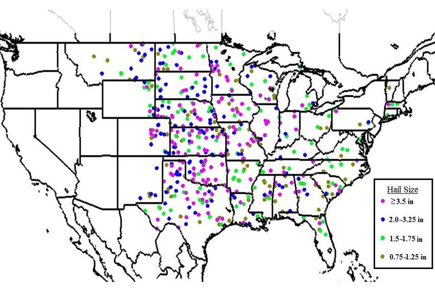
Figure 1: Hail reports from 2003, 2004, 2010, and 2011 used in this study plotted by location and size bin.
4JOHNSON AND SUGDEN 09 December 2014
To avoid duplication and subsequent biasing were obtained from the NCDC National
of the database toward cases with numerous Operational Model Archive & Distribution
reports, only the largest hail report was initially System website (http://nomads.ncdc.noaa.gov/).
included. Further, any subsequent hail reports of However, during the data-gathering phase of this
similar size were only included if they were study archived RUC analysis were missing or
beyond 6 h or 250 km from the other report. only partially available from 2005–2009.
Identical conditions apply to inclusion of smaller Despite these limitations, availability of RUC
hail except they must also pass the criteria files for 2003–2004 and 2010–2011 leaves 520
against any of the larger hailstones removed in individual hail reports. Sorting reports into the
the previous step. The 6-h and 250-km exclusion appropriate size bin, results in 152 in the ≥3.5-in
thresholds follow similar criteria used in (89-mm) range, 137 in the 2.0–3.25-in
literature such as Thompson et al. (2007) but (51–83-mm) grouping, 116 in the 1.5–1.75-in
with values increased slightly to increase (38–45-mm) range, and finally 115 in the 0.75–
confidence in removal of duplicate reports. 1.25-in (19–32-mm) collection (Fig. 1).
Despite the initial quality control criteria A change in sample size may affect the
removing numerous duplicate reports, concerns distribution of reports and statistical
involving report inclusion at smaller hail sizes interpretation of our results for a selected point
still existed. Specifically, as noted previously by granted that only a few cases exist near any
Baumgardt (2014), spotters are likely to report given location. However, while we would never
hail size to the nearest common object rather argue against a larger sample size, this study was
than the actual hailstone diameter. Unlike the still able to create a sufficiently representative
two largest hail diameter groups, the two sample size consistent with other parameter-
smallest have a narrow range of values with based climatology studies (e.g., Rasmussen and
common objects such as golf-ball hail (1.75 in, Blanchard 1998; Thompson et al. 2003; Bunkers
45 mm) sitting close to the limits of both et al. 2006).
adjacent bins. Essentially, at smaller sizes the
odds increase that we unknowingly could sort The Java-based utility, Integrated Data
some hailstones into the wrong bin. Viewer (IDV)1 was used to format and export
RUC data for interrogation by additional
Based on these concerns, this study software. RUC analysis for each report typically
strengthened the inclusion threshold for the two used a point closest to the report and the hour
smallest hail-size bins to maintain some level of valid immediately before the report time (e.g.,
uniqueness for these environments. Specifically, 21 UTC RUC analysis used for report occurring
reports passing the initial criteria but occurring at 2120 UTC). However, this process also
within 250 km and 12 h of the larger hail must be involved loading RUC surface winds, dewpoints,
within one bin size of the largest hailstone or they and surface-based (SB) CAPE in IDV to
are excluded from the database. This process diagnose any representativeness issues with the
restricts the additional inclusion criteria to ≤1.75-in analysis data. InJOHNSON AND SUGDEN 09 December 2014
14 wind-related variables remained for height along with greater magnitude above 8 km
evaluation. Further, the significant severe AGL. In contrast, the 0.75–1.25-in (19–32-mm)
parameter (SSP; Craven and Brooks 2004) and range displays noticeably weaker velocity at all
new index called the large hail parameter (LHP) levels compared to the three largest hail-size
permit evaluation of parameter combinations. bins. This difference further supports the notion
that most hail with a diameter ≥2.0 in (51 mm)
Seven of the wind-related variables are SR in requires a rotating updraft, while smaller hail
nature and require a storm motion for parameter does not (Rasmussen and Blanchard 1998;
calculation. Given the pre-storm focus of this Thompson et al. 2003; Craven and Brooks 2004;
study, observed storm motions were not Duda and Gallus 2010).
obtained, but rather the “internal dynamics (ID)
method” for predicting supercell motion The inclination toward stronger anvil-level
(Bunkers et al. 2000) was used. As detailed by flow and a slight veering profile in ≥3.5-in
Thompson et al. (2007), this method may fail for (89-mm) reports is similar to the Bunkers et al.
some elevated events and be too deviant relative (2006) composite hodograph for longer-lived
to the mean cloud-bearing winds for non- supercells. In contrast, the two middle ranges
supercell cases. Nonetheless, the majority of the look similar to the short-lived storms with
database reports still appear to be rooted in the weaker anvil-level flow and a backing profile. In
boundary layer as 85% of cases studied have addition, Rasmussen and Straka (1998) evaluated
little to no difference in CAPE between an SB supercell composite hodographs and found LP
parcel and most-unstable (MU) parcel (highest θe storms occurring in environments with stronger
value in the lowest 500 hPa). In addition, with anvil-level flow similar to hail reports ≥3.5 in
289 reports (hail ≥2.0 in, 51 mm) out of 520 total (89 mm). However, this same study also
cases likely emanating from supercells contains LP storms with unidirectional to
(Rasmussen and Blanchard 1998) and numerous backing winds above 7 km AGL similar to the
supercell cases contained within the 1.5–1.75-in two middle ranges, while winds were slightly
(38–45-mm) range, the ID method provides the veering for HP environments comparable to the
best approximation for SR parameters. largest hail-size bin. This mixed signal leaves it
unclear from hodograph shape alone, whether
3. Results: Wind-related hail reports ≥3.5 in (89 mm) occur in
environments producing lower or higher
a. Mean vertical wind structure precipitation efficiency supercells.
Initial examination of the vertical wind
structure is broken down into ground-relative
(GR) mean hodographs shown in Fig. 2 for each
of the four hail-size bins. The three largest size
categories are nearly indistinguishable in the
lowest 3 km. Further, they only begin to show
modest differences in magnitude and/or direction
starting at 4 km AGL with the largest separation
existing above 6 km AGL. Similarity in
hodograph shape and curvature below 6 km for
the larger hail sizes implies traditional wind-
based supercell parameters focusing on the
lowest 6 km may have little utility at
distinguishing between larger hail reports.
Above 6 km AGL, only subtle differences
exist between the 1.5–1.75 in (38–45 mm) and Figure 2: Composite 0–12-km AGL hodographs
2.0–3.25-in (51–83-mm) ranges as they display for each hail-size category. First three points
similar magnitude and unidirectional to slight represent surface, 0.5-km, and 1-km AGL winds
backing of winds with height. Further, between with subsequent points at 1-km intervals through
reports ≥3.5 in (89 mm) and the two middle 12 km. Stars (black rings) on the hodograph
ranges of hail size, winds in the former category represent winds at 3 km (6 km) AGL.
exhibit more of a slight veering profile with
6JOHNSON AND SUGDEN 09 December 2014 Subsequent sections will further refine some smallest range at 17 m s–1. However, more of these tendencies by examining interquartile interquartile overlap exists with these two ranges spacing. Tests of statistical significance use the compared to larger hail sizes. Student’s t-test at a 95% confidence level to determine statistically significant differences in In contrast, considerable overlap exists means (Wilks 1995). Unless otherwise noted, among the three largest hail groups with little the results were statistically significant, often separation between the two larger ranges. with p
JOHNSON AND SUGDEN                                                                       09 December 2014

from Rasmussen and Blanchard (1998) found                 composite hodographs in Fig. 2 indicate
SRH3 values discriminate supercell versus                 recognizably different structure in the upper half.
nonsupercell environments rather than tornado             The magnitude of storm-depth shear or SR wind
damage rating. Nonetheless, studies such as               above 6 km AGL has received considerably less
Rasmussen (2003), Thompson et al. (2003),                 literary attention compared to shallower, near-
Craven and Brooks (2004), Miller (2006), and              ground layers. Nonetheless, Bunkers et al.
Esterheld and Giuliano (2008), evaluate                   (2006) found the 0–8-km AGL bulk vector shear
shallower, near-ground shear layers with                  and 8-km SR winds were stronger with longer-
promising results. The magnitude of the 0–1-km            lived supercells. Further, Rasmussen and Straka
AGL bulk vector shear and SR helicity (hereafter          (1998) in evaluating supercell vertical wind
Shear1 and SRH1, respectively) were shown in              structure, found the magnitude of the 0–9-km
these studies to discriminate well between                AGL and 4–10-km AGL bulk vector shear, along
tornadic and nontornadic supercell environments.          with 9–10-km SR flow, stronger in LP versus HP
                                                          supercells. Beatty et al. (2009) also found
    Examination of SRH1 and Shear1 (not shown)            stronger upper-level SR winds with forward
reveal little interquartile separation among the          reflectivity mode supercells.
three largest binned hail sizes with any
differences not statistically significant. Further,            In evaluating upper-tropospheric winds,
SRH3 (not shown) does display some marginal               equilibrium-level (EL) calculations use a 1.5-km
difference in parameter space occupied between            non-pressure weighted mean wind. The top of
the two largest hail-size bins and the 0.75–1.25-         this layer uses an EL height derived from an MU
in (19–32 mm) cases at a value near 150 m2 s–2.           parcel with a virtual temperature correction
However, results display less interquartile               applied in the calculation (Doswell and
separation than Shear6 and ShearEff among the             Rasmussen 1994). The mean wind approach used
three largest hail groups with differences                follows results from Rasmussen and Straka
between the two largest not even statistical              (1998). Specifically, they find the strongest signal
significant. From a low-level environmental               at discriminating LP versus HP supercells occurs
wind shear perspective, tornado and maximum               with upper-tropospheric flow typically 1–2-km
expected hail size have little forecast overlap.          below the tropopause. While this study also notes
                                                          most supercells reach heights above the
d. Upper-tropospheric shear and SR wind                   tropopause, the layer approach attempts to sample
                                                          this zone of winds occurring below the EL. This
   Although development of supercell structures           process also permits sampling a broader range of
may be highly dependent on vertical wind shear            winds near anvil height than a single level.
in the lower half of a storm’s depth, the

Figure 4: As in Fig. 3 except 0–EL and 0–10-km bulk shear.

                                                      8
JOHNSON AND SUGDEN 09 December 2014
Comparison of binned hail size to storm- limited to extremely large hail. Nonetheless,
depth shear for both a fixed layer 0–10-km AGL results for ≥3.5-in (89 mm) hail lends credence
and variable depth 0–EL bulk shear (hereafter, to the assertion made by Knight and Knight
Shear10 and ShearEL, respectively) are shown in (2001) connecting lower beneficial competition
Fig. 4. In addition, Fig. 5 displays the magnitude in extremely large hail reports to stronger storm-
of the EL and 10-km AGL SR wind (hereafter, depth shear.
SRWEL and SRW10 respectively). Upper
tropospheric bulk shear using a 6 km–EL layer e. Lower- and mid-tropospheric SR wind speed
(hereafter Shear6–EL) is calculated but not shown.
Unlike Shear6, Shear10 and ShearEL display some Through analysis of over 250 observed
interquartile separation at around 25–30 m s–1 proximity soundings, Maddox (1976) found
between the two largest binned hail sizes with tornadic storms to display similar lower-to-mid-
these differences statistically significant. tropospheric SR winds compared to nontornadic
However, more overlap exists among the three storms. Later research by Brooks et al. (1994a)
smallest binned hail sizes compared to Shear6, and Beatty et al. (2009) discovered a modest
especially with 0.75–1.25-in (19–32-mm) cases relationship between stronger mid-tropospheric
versus larger hail sizes. SR winds and supercells favoring an LP and
forward reflectivity mode. Other studies such as
Examination of Shear6–EL (not shown) along Rasmussen and Straka (1998) found the opposite
with SRWEL, and SRW10 in Fig. 5 further display to be true while Bunkers et al. (2006) found little
this relationship. Events ≥3.5 in (89 mm) connection with either lower or mid-tropospheric
partially occupy different parameter space SR winds and supercell longevity. Further,
starting at values around 8 m s–1 for Shear6–EL Thompson (1998) revealed midtropospheric SR
and 16 m s–1 for SRWEL and SRW10. In contrast, winds stronger in tornadic supercells compared
considerable overlap exists among the three to nontornadic. However, research by Thompson
smallest hail groups with any differences not et al. (2003) uncovered the difference in the
statistically significant. These results suggest the mean mid-tropospheric SR winds was too small
sphere of influence of storm-depth shear or SR to make it a suitable parameter for discriminating
winds on maximum potential hail size may be significantly tornadic and nontornadic supercells.
Figure 5: As in Fig. 3 except EL and 10-km SR wind magnitude.
9JOHNSON AND SUGDEN 09 December 2014
Figure 6: As in Fig. 3, but EL GR wind & 3–6-km GR wind direction difference.
Figure 7: As in Fig. 3, but 3–6-km SR wind & 0–1-km SR wind direction difference.
The 0–1 km and 3–6-km SR wind magnitude among the three largest groups with no statistical
(hereafter, SRW1 and SRW3–6 respectively) are significance existing between the two largest size
calculated but not shown. SRW3–6 reveals little, ranges.
if any, parameter spacing among all bins. In
contrast, a modest relationship exists in SRW1 This relationship is not only similar to that
between the two largest hail-size bins and the shown by Shear6 and ShearEff at separating
0.75–1.25-in (19–32-mm) cases as they occupy a obvious supercell reports (≥2.0 in, 51 mm) from
different portion of the parameter spaceat around more mixed-mode cases (≤1.25 in, 32 mm), but
11–12 m s–1. However, extensive overlap exists also highly correlated (Table 1). It may initially
10JOHNSON AND SUGDEN 09 December 2014
appear odd that SRW1 is highly correlated to a duplicate wind layers used by SRWαMid and
shear value but near-surface SRW layers are Shear6 result in very similar skill in separating
highly influenced by storm motion. With the ID more obvious supercell cases from mixed-mode
technique dependent on winds in the 0–6-km cases.
layer, a near duplication of wind layers used
either directly with Shear6 and ShearEff or 4. Results: Thermodynamic-related
indirectly with SRW1 creates similar results.
Further, SRW1 values occur in a narrow range a. MUCAPE and MLCAPE
well within the margin of error of NWP. Both of
these latter relationships leave SRW1 with CAPE is a measurement routinely used by
limited potential as a hail-forecast tool. operational forecasters to estimate environmental
thermodynamic instability, where larger values
f. Lower and upper tropospheric wind direction correlate with the potential for greater updraft
velocity. However, this method is very inaccurate
As briefly discussed in section 3a, notable at predicting maximum updraft velocity and hail
wind direction differences exist among the hail- size as discussed by Doswell and Markowski
size bins, especially above 6 km AGL. (2004). As detailed with EL height, computed
However, most studies looking at the vertical CAPE uses a vertical thermal profile with a
wind structure in relation to severe convection virtual temperature correction applied (Doswell
generally focus on parameters providing the and Rasmussen 1994).
magnitude of either the vertical wind shear or SR
wind. Browning (1977) found that it may be As previously detailed in Section 2, the
critical for the wind direction difference, α, majority of cases studied have little to no
between the SR low-level inflow and mid-level difference between SBCAPE and MUCAPE.
flow, be at least perpendicular in order to deliver However, for the ≈15% of cases that occur with
hail embryos to a location where they can be a relatively stable near-surface layer, MUCAPE
ingested into the updraft. provides some estimation of elevated instability
encountered by these storms that is not well-
Figure 6 further examines α above 6 km resolved in a surface value. Nonetheless, rather
AGL, by using a simple subtraction of the GR than examining only the highest CAPE in the
EL wind direction and GR 3–6-km wind lowest 500 hPa without any consideration for
direction (hereafter, GRWαEL). Evaluating Fig. 6 entrainment of more stable air, evaluation of
from a parameter space perspective displays CAPE also includes a mixed-layer (ML) CAPE
significant overlap among the four binned hail- that uses a parcel with a uniformly mixed
size groups. However, similar to the tendencies equivalent potential temperature in the lowest 50
seen in the composite hodographs, extremely hPa. The 50-hPa mean parcel layer was chosen
large hail reports (≥3.5 in, 89 mm) display a over the commonly used 100-hPa depth (Craven
propensity toward a slight veering wind profile et al. 2002b) to better represent shallow moisture
(positive values) above 6 km. Although far from layers (JOHNSON AND SUGDEN 09 December 2014
surface. Further, their boundary layer corrective issues or a combination results in this difference
scheme also uses the maximum regional surface is unknown, yet a signal toward a MUCAPE or
temperature and dewpoint value found in the MLCAPE ≥2000 J kg–1, is seen in hail reports
inflow air but also results in the upper limit of ≥3.5 in (89 mm) compared to smaller sizes.
expected values. Which of these potential bias
Figure 8: As in Fig. 3 except total MUCAPE and MLCAPE.
Figure 9: As in Fig. 3 except –10˚C to –30˚C and 3–6-km AGL MUCAPE.
12JOHNSON AND SUGDEN 09 December 2014
b. Hail-growth-zone parameters c. Lapse rates
The hail-growth zone (HGZ) as defined by Craven and Brooks (2004) have shown that
studies such as Nelson (1983), Foote (1984), significant severe weather events have steeper
Miller et al. (1988), and Knight and Knight 700–500-hPa lapse rates (hereafter, LR7–5) than
(2001), occurs within a layer bound by –10˚C marginal severe or non-severe events. However,
and –30˚C. Most forecast techniques looking at that study combines hail and wind reports into
this layer are generally radar-based applications one category, with any hail signal possibly
such as from Blair et al. (2011). Nonetheless, a obscured by wind reports. Figure 12 in this
few studies such as Fawbush and Miller (1953), study provides a direct comparison of binned
Miller (1972), and Moore and Pino (1990), hail size against LR7–5.
evaluate various measures of instability generally
below this layer as predictors for hail size. LR7–5 displays considerable overlap similar to
However, techniques developed from this CAPEHGZ, and to a lesser degree, other
literature display marginal skill at forecasting thermodynamic-related parameters discussed
maximum hail size with results frequently previously. Nonetheless, a tendency toward
overestimating diameters (Doswell et al. 1982). steeper lapse rates exists between the smallest
binned hail sizes and the two largest at around
Figure 9 investigates instability within the 6.5–7.0˚C km–1. However, little interquartile
HGZ and in a region typically just below by spacing exists between the two larger hail sizes
looking at MUCAPE in the –10˚C to –30˚C and or between the two smaller groups with
3–6-km AGL layers (hereafter, CAPEHGZ and differences in either pairing failing in statistical
CAPE3–6 respectively). CAPE3–6 depicts little significance. Examining lapse rates in layers
interquartile separation among the groups above 700–500 hPa (not shown) reveal similar
although only the two largest hail-size bins results. The 500–300-hPa and HGZ lapse rates
have differences that fail in statistically (hereafter, LR5–3 and LRHGZ respectively),
significance. CAPEHGZ displays much of the display a similar tendency toward slightly
same statistical significance and slight tendency steeper lapse rates as binned hail size increases
to occupy different parameter space as hail size but with only minor interquartile separation.
increases but still with substantial overlap.
Further, comparing CAPEHGZ to MUCAPE and d. Significant height levels
MLCAPE reveals the former displaying less
interquartile separation than the total CAPE Rasmussen and Blanchard (1998),
parameters. Markowski et al. (2002), Thompson et al. (2003),
and Craven and Brooks (2004) found the lifted
A method to view this relationship is to condensation level (LCL) height discriminates
compare the percentage of total MUCAPE well between significant tornadic supercell
existing only in the HGZ (hereafter, %CAPEHGZ) events and those that are only weakly tornadic
against the four hail-size groups (Fig. 10). or nontornadic. However, aside from the
Although little signal is shown for 0.75–1.25-in significant tornadic cases, these studies also
(19–32-mm) reports versus larger sizes, a reveal that the LCL height has little additional
noticeable tendency is seen when looking at utility among all other groups, including little
reports in the three largest hail-size bins. skill at differentiating severe and non-severe
Specifically, comparing the three largest groups environments. Evaluation of MULCL in this
against each other reveals an inverse relationship study (not shown) reveals little, if any,
with a lower percentage of total MUCAPE interquartile spacing with any differences failing
residing within the HGZ as hail sizes become in statistical significance.
larger. Another method to examine this finding
is to compare the HGZ thickness (hereafter, Environmental freezing level (FZL) and wet-
THKHGZ) to the hail-size bins. Figure 11 reveals bulb zero (WBZ) heights have become common
a similar inverse tendency in THKHGZ versus hail tools when combined with radar for hail
size, especially with ≥3.5-in (89-mm) diameter prediction (e.g., Donavon and Jungbluth 2007).
hail. In addition, the differences in the means Nonetheless, these techniques provide limited
among the three largest hail-size bins all are value prior to storm formation. Miller (1972)
statistically significant for THKHGZ. attempted to use environmental FZL information
with various measures of buoyancy to create a
13JOHNSON AND SUGDEN 09 December 2014
Figure 10: As in Fig. 3 except percent of total MUCAPE in HGZ.
Figure 11: As in Fig. 3 except HGZ thickness.
Figure 12: As in Fig. 3 except 700–500-hPa lapse rate.
14JOHNSON AND SUGDEN 09 December 2014
predictive tool for hail size. However, AGL bulk vector shear. However, neither of
application of these techniques typically reveal these studies evaluates ESI directly against
very limited success, and attempting to use FZL binned hail sizes but rather as a measure of
and/or WBZ alone as a predictive tool results in updraft duration in HAILCAST.
even less skill (Kitzmiller and Briedenbach
1993; Edwards and Thompson 1998). Yet another CAPE-shear combination called
Examining FZL and WBZ heights against the the significant hail parameter (SHIP; SPC 2014)
hail-size bins (not shown) only further reinforce is an index developed in-house at the SPC.
results from these earlier studies. Specifically, Unlike SSP and ESI, SHIP includes more than
little interquartile separation exists between the just CAPE and shear. Three additional variables
hail groups with any differences failing in are part of the formula and include the mixing
statistical significance. ratio of a MU parcel, the LR7–5, and 500-hPa
temperature that appear to help SHIP delineate
5. Results: Parameter combinations between ≥2.0-in (51-mm) hail and smaller sizes.
While the SHIP formula specifically targets hail
a. Significant severe parameter (SSP) discrimination rather than other severe-
convective elements, evaluation of SHIP has not
Various combinations of instability and shear undergone a prior literary review with
have been created over the years to assist in performance against multiple binned hail sizes
forecasting severe-convective potential. Popular unavailable. Further, a skewing of results may
parameter combinations such as the energy- exist (SPC 2014) by the removal of all 1.75–
helicity index (EHI; Hart and Korotky 1991; 2.0-in (45–51-mm) reports in order to magnify
Davies 1993), vorticity generation parameter interquartile separation.
(VGP; Ramussen and Wilhelmson 1983), and
both the supercell composite parameter and Not all parameters needed for calculation of
significant tornado parameter (SCP and STP, ESI and SHIP are examined in this study.
respectively; Thompson et al. 2002a,b, 2003) However, those needed for SSP are available
have focused on varying degrees of supercell with results following below. Unlike the Craven
and/or tornado prediction. However, most of and Brooks (2004) study blurring hail and wind
these parameters exist with little, if any, literary reports together, SSP results for hail only cases
attention given toward hail prediction although a (Fig. 13) reveal overall better interquartile
few exceptions exist. separation among the four original binned hail
sizes (left side of Fig. 13) than any of the
Craven and Brooks (2004) evaluate SSP individual variables. The best tendency in
against significant tornado events, significant interquartile separation among the four groups
and non-signficant wind and/or hail cases, and exists between two smallest ranges and the
general- or no-thunder cases with the index largest hail-size bin at a value of 40 000–
formula following: 45 000 m3 s–3. On the other hand, marginal
severe cases ≤1.25 in (32 mm), and reports
SSP = (MLCAPE J kg –1)*(Shear6 m s –1) deemed “significant” from other literature in the
2.0–3.25-in (51–83-mm) range, display a more
As the product of MLCAPE and Shear6, modest level of interquartile separation, with
Craven and Brooks (2004) SSP displays some little improvement over Shear6 or ShearEff.
skill at distinguishing between cases with ≥2.0-in Further, similar to Shear6 and MLCAPE,
(51-mm) hail and/or ≥65-kt (33.4-m s –1) winds considerable overlap exists between the two
versus reports with smaller hail and/or lesser larger hail-size bins although unlike Shear6
wind. However, hail-only categories were not differences are statistically significant.
constructed. This leaves any potential hail signal
blurred with wind reports that may have little In order to make a more direct comparison to
significant hail. the figures given by SPC (2014) for the SHIP
index, two additional hail-size bins are included
A similar CAPE-shear combination called the on the right side of Fig. 13 comparing reports
energy shear index (ESI; Brimelow et al. 2002) ≤1.25 in (32 mm) with those ≥2.0 in (51 mm).
is part of the HAILCAST model algorithm Although with slightly more overlap than SHIP,
(Jewell and Brimelow 2009), and is the product SSP displays very similar results with good
of SBCAPE and magnitude of the 850 hPa–6-km interquartile separation among ≤1.25-in (32 mm)
15JOHNSON AND SUGDEN 09 December 2014
Figure 13: As in Fig. 3 except SSP and inclusion of two extra binned hail sizes.
reports and ≥2.0-in (51-mm) cases. The nearly As expected, wind-related variables in
identical results should not be surprising since Table 1 have strong independence with the
both SHIP and SSP use Shear6 and some variation thermodynamic-related variables. Given this
of CAPE. However, it becomes apparent when reality, use of any parameter from one of these
reviewing the left side of Fig. 13 that most of the groups depends more on selecting those
interquartile spacing existingwith SSP is not from variables displaying at least some interquartile
delineating environments producing ≥2.0-in separation along with strong independence
(51-mm) hail versus smaller sizes, but only from among related variables. Most of the shear and
environments that will produce ≥3.5-in (89-mm) storm-relative wind variables have a strong
hail. The fact that the 2.0–3.25-in (51–83-mm) interdependence (higher correlation coefficient)
range still modestly overlaps the two adjacent among each other, especially when comparing
hail-size bins along with nearly 50 percent of layers of similar depth (e.g., 0.94 for ShearEff and
cases in the smallest hail range raises questions on Shear6). Further, GRWαEL and to a lesser degree
the validity of forecasting ≥2.0-in (51-mm) hail SRWαMid display independence in comparison to
from smaller sizes using SSP or SHIP. The most other wind variables while also exhibiting
question then becomes whether adding any some notable parameter spacing differences as
additional parameters from sections 3 and 4 to a discussed in section 3.
simple CAPE-shear combination would improve
interquartile separation and subsequent predictive Among the thermodynamic parameters
capability. displaying strong interquartile separation, most
of the MUCAPE variables have high
b. Large hail parameter (LHP) interdependence. This relationship only further
reinforces results from section 4 indicating
One of the first steps in evaluating additional measurements of CAPE in or near the HGZ
parameter combinations is selecting from those provide little improvement over CAPE. In
variables displaying at least some interquartile contrast, MUCAPE has a strong independence
separation, as discussed in previous sections. with 1) LR7–5 and 2) unconventional measures
However, these same parameters must also have such as THKHGZ. Further, combinations of these
strong independence (low correlation coefficient) thermodynamic indices with the aforementioned
among the variables included, to avoid overly wind parameters may yield some improvement
strong influence from just one set of related over a simple CAPE-shear combination such as
parameters. Table 1 displays a correlation matrix SSP.
for most of the variables listed in sections 3–4.
16JOHNSON AND SUGDEN 09 December 2014
Table 1: Correlation matrix for 17 of the 26 parameters evaluated in the present study. The digits across the top row correspond to the numbered fields on the
side. See sections 3 and 4 for a definition of the parameters.
1 2 3 4 5 5 7 8 9 10 11 12 13 14 15 16 17
1) Shear6 1.0
2) ShearEff 0.94 1.0
3) SRH1 0.50 0.50 1.0
4) SRH3 0.50 0.50 0.87 1.0
5) Shear10 0.77 0.75 0.31 0.33 1.0
6) ShearEL 0.75 0.73 0.32 0.33 0.89 1.0
7) SRW10 0.38 0.37 0.01 0.04 0.84 0.69 1.0
8) SRWEL 0.30 0.29 –0.02 0.00 0.67 0.80 0.80 1.0
9) SRWαMid 0.62 0.63 0.33 0.45 0.51 0.51 0.26 0.22 1.0
10) GRWαEL 0.21 0.21 0.19 0.17 0.20 0.25 0.00 0.02 –0.01 1.0
11) MUCAPE –0.28 –0.19 –0.12 –0.13 –0.28 –0.23 –0.20 –0.11 –0.12 –0.06 1.0
12) MLCAPE –0.26 –0.18 –0.17 –0.16 –0.25 –0.20 –0.18 –0.11 –0.13 –0.03 0.88 1.0
13) CAPEHGZ –0.20 –0.12 –0.12 –0.11 –0.18 –0.13 –0.09 –0.01 –0.04 –0.06 0.94 0.82 1.0
14) CAPE3–6 –0.22 –0.15 –0.16 –0.18 –0.18 –0.13 –0.08 0.00 –0.08 –0.07 0.87 0.76 0.92 1.0
15) %CAPEHGZ 0.24 0.22 0.09 0.12 0.31 0.25 0.28 0.19 0.19 –0.03 –0.36 –0.34 –0.16 –0.19 1.0
16) LR7–5 0.24 0.26 0.10 0.18 0.26 0.29 0.19 0.21 0.29 0.12 0.19 0.20 0.34 0.28 0.25 1.0
17) THKHGZ –0.03 –0.04 –0.04 –0.05 0.00 –0.06 0.06 –0.02 –0.04 –0.10 –0.10 –0.14 0.06 0.04 0.25 –0.10 1.0
17JOHNSON AND SUGDEN 09 December 2014
Before discussing creation of a new percentile values for the three largest hail-size
parameter (LHP), a review on the limitations of bins shown in Fig. 4. This lower limit not only
parameter combinations is necessary. Doswell provides a small buffer below the ≈17-m s–1
and Schultz (2006) address how most indices are threshold for the three largest hail-size bins, but
diagnostic rather than prognostic in nature. In also fits well with the Thompson et al. (2002a,b,
particular, these indices only identify the current 2003) findings pointing to most supercell cases
state of the atmosphere with no established with values of Shear6 ≥15–20 m s–1.
predictive quality of future weather. Like many
other composite parameters, LHP and SSP are Given this Shear6 limit, the formula checks if
not exempt from being diagnostic. With no values are ≥14 m s–1 and if false, the LHP sets to
established predictive quality outside of an zero with no further calculations made. Further,
NWP-derived value, LHP and SSP cannot make to avoid unnecessarily high LHP values in
predictions of future weather without regard to weakly unstable environments, the formula also
the state of the atmosphere at that forthcoming checks if MUCAPE values are ≥400 J kg–1 and if
time (Doswell and Schultz 2006). However, by false, LHP sets to zero. A MUCAPE of
understanding these limitations an observed or 400 J kg–1 was chosen as a lower limit since this
NWP-derived LHP, along with deeper analysis, correlates to the 10th percentile value for 0.75–
can provide a full picture of potential hail sizes. 1.25-in (19–32-mm) reports shown in Fig. 8 and
is slightly below the 5th percentile for the two
To evaluate performance of including the largest hail-size bins (not shown).
aforementioned variables in a CAPE-shear
combination, construction of a new parameter is If both of these checks pass then five new
required. The unitless LHP includes CAPE and variables along with MUCAPE create the LHP.
shear but also a combination of other These variables are broken down into a
thermodynamic and wind-related variables thermodynamic and wind-related component.
displaying some predictive skill. The LHP The product of these two elements along with a
formula is as follows: small addition term, create the parameter value.
The thermodynamic component (Term A) is
If Shear6 magnitude < 14 m s–1 OR composed of MUCAPE, THKHGZ, and LR7–5.
MUCAPE < 400 J kg–1: Each of these variables displays modest
interquartile separation and strong independence
LHP = 0 among each other. The wind-related component
(Term B) is composed of a ShearEL, GRWαEL,
If Shear6 magnitude ≥ 14 m s–1 AND and finally SRWαMid. If GRWαEL is >180˚, this
MUCAPE ≥ 400 J kg–1: portion of Term B is set to –10 as to avoid
incorrectly labeling a small backing wind profile
LHP = (Term A * Term B) + 5 as strongly veering. Further, a value of 5 added
Term A = (((MUCAPE – 2000)/ 1000) + to the end of the LHP formula creates more
((3200 – THKHGZ)/500) + separation for index values near zero that were
((LR7–5 – 6.5)/2)) derived after the initial Shear6 check passes
versus leaving LHP at zero when the initial
Term B = (((ShearEL – 25)/5) + checks fail. Additionally, if Term A and B are
((GRWαEL + 5)/20) + both negative the LHP is set to zero to avoid
((SRWαMid – 80)/10)) creating a positive value by multiplying two
negative terms. Finally, if values are still not
An explanation of each portion of the above zero after the previous addition term, all
parameter is necessary to understand reasoning negative values of the LHP are set to zero.
behind the formula. Unlike most traditional
CAPE-shear combinations using either Shear6 or Evaluation of LHP in Fig. 14 reveals
ShearEff as a CAPE multiplier, results from improvement over SSP, especially between hail
section 3b indicate Shear6 is better suited as a reports in the 2.0–3.25-in (51–83-mm) range
simple toggle for supercell potential and versus the smallest hail-size bin. At a value of 4–
subsequent threat of ≥2.0 in (51 mm) hail. Use 6, these two ranges now appear to occupy a
of 14 m s–1 as a lower limit correlates to the different portion of the parameter space in contrast
median value for 0.75–1.25-in (19–32-mm) to SSP. Further, improvement also exists over
reports and is slightly below the 10th and 25th SSP between the two smallest groups and the
largest hail-size bin at an LHP value of 7–8.
18JOHNSON AND SUGDEN 09 December 2014
Figure 14: As in Fig. 3 except LHP and inclusion of two extra binned hail sizes.
Examining the right side of Fig. 14 for reports between SSP and Shear6, CAPE apparently adds
also depicts improvement in interquartile spacing little predictive skill at this range of hail sizes.
of ≥2.0-in (51-mm) versus ≤1.25-in (32-mm) cases
over SSP. Nonetheless, with only minor As intriguing as LHP skill initially appears in
improvement among the three larger hail sizes, this size range, skill at such a sharp delineation in
the increased parameter spacing in LHP between hail sizes is misleading. By examining the other
the two smallest groups and the largest hail-size columns (b–d), skill gained in separating ≥2.0-in
bin is likely coming through better delineation of (51 mm) hail from smaller sizes is not by
the 2.0–3.25 in (51–83-mm) and 0.75–1.25-in differentiating the two middle hail-size groups
(19–32-mm) ranges mentioned earlier. The use (column b). On the other hand, given the
of Shear6 as a simple toggle for larger hail parameter-space overlap between these binned
potential rather than as a CAPE multiplier hail sizes, simply replacing 1.5–1.75-in (38–
appears to improve hail predictive capability via 45-mm) reports with 0.75–1.25-in (19–32-mm)
this two-step process. cases (column c) allows skill to increase for some
parameters. LHP, Shear6 and SRWαMid display
Analysis of parameters so far in this study the highest HSS while other parameters including
provides only a perceived skill by examination SSP are lower in skill.
of interquartile spacing in box and whisker plots.
To bridge this evaluation gap, Table 2 displays Despite the lack of predictive skill at such
the Heidke’s skill score for selected parameters narrow ranges of typical supercell hail sizes, the
(HSS; Doswell et al. 1990). An HSS value of 1.0 interquartile separation shown between reports
is a “perfect” forecast while valuesJOHNSON AND SUGDEN 09 December 2014
Table 2: a) Parameters ranked according to Heidke’s skill score for all reports based on the threshold value
given for ≥2.0 in (51 mm) hail size prediction. b) Same as (a) but with the largest and smallest hail size
reports excluded. c) Same as (a) but with the largest bin and 1.75–2.0-in (45–51-mm) reports excluded.
d) Same as (a) but with the smallest bin and 2.0–3.25-in (51–83-mm) reports excluded and based on the
threshold value given for ≥3.5-in (89-mm) hail-size prediction.
(a) (b) (c) (d)
All Reports Excluded Excluded Excluded
0.75–1.25 in 1.5–1.75 in 2.0–3.25 in
≥3.5 in ≥3.5 in 0.75–1.25 in
Parameter Threshold Value HSS HSS HSS HSS
≥2.0 in | ≥3.5 in ≥2.0 in ≥2.0 in ≥2.0 in ≥3.5 in
LHP 5|7 0.47 0.26 0.49 0.52
3 –3)
SSP (m s 30,000 | 40,000 0.39 0.23 0.38 0.41
–1
Shear6 (m s ) 20 | 22 0.32 0.19 0.41 0.24
–1
ShearEL (m s ) 24 | 29 0.28 0.11 0.27 0.30
–1
MUCAPE (J kg ) 1,850 | 2,700 0.18 0.12 0.07 0.24
–1
LR7–5 (˚C km ) 6.5 | 7.0 0.33 0.22 0.32 0.35
THKHGZ (m) 3,100 | 3,000 0.17 0.14 0.03 0.31
GRWαEL (˚) –5 | 0 0.17 0.14 0.14 0.23
SRWαMid (˚) 80 | 90 0.38 0.27 0.47 0.28
6. Conclusions and summary ShearEL, display less of a signal at the lower end
of hail sizes yet better skill at delineating ≥3.5-in
A large-hail report database created in this (89-mm) hail from smaller sizes. Although
study uses Storm Data reports from the years of overall skill of GRWαEL remains low, results
2003, 2004, 2010, and 2011. Through various indicate that for ≥3.5-in (89-mm) hail to occur,
quality-control measures, 520 remaining hail winds in the upper half of a storm’s depth should
reports sort into one of four hail-size categories. veer or back only slightly with height. In the
From these cases, extraction of numerous RUC lower half of a storm's depth, SRWαMid veers by
sounding-derived fields creates a parameter- no less than 80–90˚ in most ≥2.0-in (51-mm)
based climatology of hail reports. hail-size reports.
Initial examination of mean composite MUCAPE and MLCAPE along with LR7–5
hodographs indicate a weaker vertical wind display a slight upward tendency in values and
structure with the smallest hail-diameter range in resultant skill as hail size increase but still with a
comparison to the three largest bins. However, considerable amount of overlap. Shallower
among the three largest hail-size bins, the layers of instability such as CAPEHGZ and
vertical wind structure is nearly indistinguishable CAPE3–6 reveal less interquartile separation than
in the lowest 3–4 km but then displays total MUCAPE. Further, %CAPEHGZ and
differences above 6 km AGL. The ≥3.5-in THKHGZ display an inverse relationship with hail
(89-mm) cases reveal the most notable difference size with values decreasing as diameters
via a slightly more veering profile along with a increase. Significant height levels such as FZL,
greater wind magnitude. WBZ, and LCL reveal little if any interquartile
spacing or skill to discriminate among the hail-
Additional inspection of wind-related size bins. The poor performance of FZL and
parameters simply reinforce tendencies shown in WBZ is similar to Edwards and Thompson
the mean hodograph, as lower shear layers such (1998) and raises questions on the validity of
as Shear1 or SRH1 reveal little if any parameter using them in severe-convection forecasting
spacing among all hail sizes. Surface-to-mid- despite common use in radar-based interrogation.
level shear layers such as Shear6 reveal modest
skill at discriminating the smallest hail-size bin The new parameter combination LHP, and to
from the two largest, but with little ability to a lesser degree SSP, show the strongest ability to
distinguish between the three largest hail-size discriminate between hail-size bins. When
bins. In contrast, much deeper shear such as delineating ≥2.0-in (51-mm) hail cases versus
20JOHNSON AND SUGDEN 09 December 2014
smaller sizes, LHP displays improved skill and quickly into extremely large hail sizes.
interquartile separation over all individual Nonetheless, this is only one of many
parameters, including SSP. However, when mechanisms that can result in lower beneficial
comparing 2.0–3.25-in (51–83-mm) reports to competition needed for larger hail growth. In
the smallest hail-size bin, LHP and SSP skill is addition, some of this relationship might also
similar or lower than SRWαMid and Shear6. In relate to nonhydrostatic vertical pressure
contrast, skill for SRWαMid and Shear6 drop gradients induced by the rotating updraft as Blair
when comparing ≥3.5-in (89 mm) reports to 1.5– et al. (2011) reveal a strong correlation between
1.75-in (38–45-mm) cases, while SSP and LHP mid-level rotational velocity and hailstone size.
skill increase. An area of future work that may
result in additional skill for the LHP is to switch Results do not suggest any reasonable
from Shear6 to ShearEff while adjusting SRWαMid capability through parameter analysis alone to
to use winds from this same effective layer. To discriminate 2.0–3.25-in (51–83-mm) reports
compare successfully an effective layer LHP to from the adjacent larger and smaller hail-size bins.
the fixed layer version requires a refinement and These narrow ranges of hail size are nearly
subsequent binning of reports emanating from indistinguishable from each other with low
elevated convection. However, this level of predictive skill existing. Even when broadening a
convective detail is unknown in this study. range to better detect ≥3.5-in (89-mm) hail,
upstream convection may create anvil ice seeding
The implication of these results is that once that ultimately suppresses large hail development
the environment becomes favorable for rotating due to increased competition for supercooled
updrafts, the role of traditional supercell-based water (Knupp et al. 2003). Additional refinement
indices such as Shear6 to dictate production of or narrowing of results would have to be
≥3.5-in (89-mm) hail diminishes. In contrast, the accomplished through prediction of convective
role of items associated with storm-precipitation mode and duration, hail growth models such as
efficiency, updraft strength, and storm longevity HAILCAST (Jewell and Brimelow 2009), and/or
such as ShearEL, THKHGZ, GRWαEL, and other methods yet to be deployed.
MUCAPE, increase. Essentially, once the
supercell box toggles to “yes” results outlined This study raises many questions as to the
suggest a forecast of maximum hail sizes at any physical explanation behind some of the
diameter ≥1.5 in (38 mm) is within the bounds of parameter trends shown. The answers to these
reality. However, the next step involving various questions are well beyond the scope of this study
non-traditional parameter combinations assists without extensive modeling and/or analysis of
with discriminating ≥3.5-in (89-mm) hail from storm microphysics in field projects. However,
smaller sizes. predictability problems will likely always exist.
Further, hail embryo trajectories and subsequent
The counter intuitive results of parameters in growth into a hailstone is complex and
or near the HGZ suggest the depth of this layer dependent on processes not easily resolved in
becomes shallower for larger binned hail sizes operational meteorology or modeled soundings.
but with no significant increase in layer Nonetheless, future projects may build on this
instability. In addition, with CAPE increasing as study’s climatology to create new predictive
hail size becomes larger, the lack of a similar tools for hail-size discrimination.
change in instability within and below the HGZ
imply higher CAPE is occurring above this layer. ACKNOWLEDGMENTS
Although the exact mechanism resulting in this
relationship is unknown, Knight and Knight The authors wish to express their
(2001) discuss the impacts on hail growth by appreciation to Larry Ruthi and Mike Umscheid
modification of storm-precipitation efficiency (NWS Dodge City, Kansas) for technical editing
and resultant beneficial competition. This type of and assistance with computer scripting. We
setting may produce a higher percentage of would also like to thank Roger Edwards (SPC),
nascent hail embryos prematurely ejecting into John T. Allen (IRI, Columbia University), Scott
the anvil due to inadequate growth time and Blair (NWS), and Jeff Manion (CRH) for their
higher parcel ascent above the HGZ. helpful reviews and thorough copyediting. The
Conceptually, this would leave only a few views expressed within this manuscript are those
remaining hail embryos with unfettered access to of the authors and do not necessarily represent
supercooled water and increased ability to grow those of the National Weather Service.
21You can also read