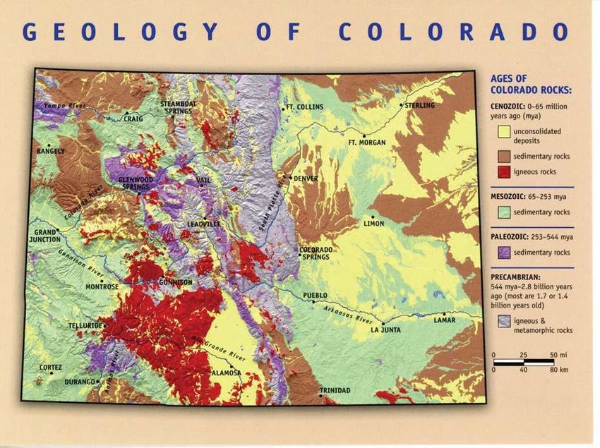
Exercise 6 Time distribution of rocks in Colorado: Colorado Geologic Map, Tweto 1979.
←
→
Page content transcription
If your browser does not render page correctly, please read the page content below
Geol 3050 – GIS for Geologists – Exercise 6

Exercise 6 Time distribution of rocks in Colorado:
Colorado Geologic Map, Tweto 1979.
Due: Thursday, February 7, 2019.
Goal: Query datasets, recalculating tables and dissolving a file.

Datasets: to be downloaded from the USGS

Assignment

The Colorado Geological Survey (CGS) has created a series of maps showing the age
distribution of rocks in Colorado, based on the 1:500,000 geologic map of our state. By using a
reclassification of the original data we are going to make a similar set of maps. Study the example
map below:

                                                        1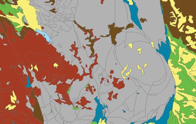
Geol 3050 – GIS for Geologists – Exercise 6

IMPORTANT: We have discussed best practices for saving and storing your data and maps (they are
different! Remember?). In this lab this will be important, as you will be using your results from this lab
for our next exercise. Keep your data (including all your ArcMap tool outputs) and map files together,
and make sure they are stored somewhere that you can access next week. As always, remember to
“Store relative pathnames”. Everything to be turned in is listed at the end of the exercise.

 Part A. Setup your map:

     1. Open ArcMap.
     2. Go to: https://mrdata.usgs.gov/geology/state/state.php?state=CO
        download the shapefile (COgeol_dd.zip).

 1. Save and Unzip your file Colorado.zip to your flash drive or D:\myGIS\Exercise6 folder or flash
 drive.

 2. In ArcCatalog, browse your data (If you don’t see your new data, try to refresh your screen) (use
 the cogeol_polygon_dd.shp file):

 3. Check out what you got by right clicking on the file and selecting “Item Description…”: do a
 preview (something you notice on the shape?) and View Metadata: Select the cogeol_dd file in
 Catalog and go to the “Description” Tab. This is where your Metadata should be! From the
 ArcCatalog file menu, choose Customize -> ArcCatalog Options, and select the “Metadata” tab.
 Under “Metadata Style”, choose “ISO 19139 Metadata Implementation Specification” and click OK.
 Then, go look in the “Description” Tab.

 4. Go to the Shapefile Properties (See exercise 5 for reference if you forgot)

 5. Go to XY coordinate System (this is an alternate way of defining the coordinate system than we
 used in Exercise 5, item 20)

 6. Make sure that the projection is Geographic > North America > North American Datum 1927.

 7. Go back to your webbrowser and find the page where you downloaded the geologic map of
 Colorado (https://mrdata.usgs.gov/geology/state/state.php?state=CO )

 8. However, now try to find out more about the projection via the metadata online and compare it to
    the metadata displayed in ArcCatalog.

 9. (search for "projection").

 10. Go to Spatial_Ref_Info: How does the data set represent geographic features?
                                                 2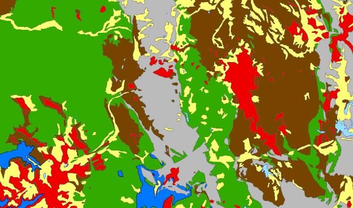
Geol 3050 – GIS for Geologists – Exercise 6

11. Find out more about the map projection details. Keep this window open so you can copy this
information later on.

12. Open ArcToolbox

13. Go to Data Management Tools > Projections and Transformations > Project.

14. Name the new file cogeology1_project.shp
15. For the output coordinate system, use the information you just found in the metadata:
Projected Coordinate Systems > Continental > North America
> USA Contiguous Lambert Conformal Conic

Do NOT hit ok yet!

16. Instead, double click on the projection (USA Contiguous Lambert Conformal Conic):

                                                        3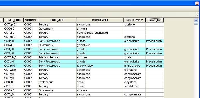
Geol 3050 – GIS for Geologists – Exercise 8

17. When you check your information (hopefully still open in your web browser) with the XY
coordinate system information you just set, you will see some differences in the Central Meridian,
AND the datum!

18. So, it is not always good to just go with the defaults!

19. We will reset these values to what works for our map.

20. Reset the Central Meridian value to -105.5 degrees (see image on next page).

21. Modify the value for the Geographic Coordinate system (this is your datum) as we need NAD
1927 and not NAD 1983 (both in General/Name and Datum/Name:

This will automatically reset the correct ellipsoid.

22. Browse to North America > North American Datum 1927

23. Click 1 time and then OK then OK again then OK again. (If you get an error then you will
have to remove the default transformation for it to run smoothly.

                                                          4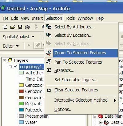
Geol 3050 – GIS for Geologists – Exercise 8

 You have now reprojected your file so it centers on Colorado (-105.5 degrees west from Greenwich
(instead of -96 degrees near Kansas City, which is often used for the entire continental US) on a
1927 datum)! You will now need to open a blank copy of ArcMap and add the projected file!

Adjusting the symbology:

    3. There is no symbology defined in this downloaded file.
    4. Go to Layer Properties and adjust the symbology:
           • Categories > Unique Values (Remember how to add these values?)
           • Color Scheme = Random colors
           • Value field = ORIG_LABEL
           • Add all Values
           • Click OK

Notice that we now have many classes defined\colored, there is a need to summarize what we see to see
where rocks of which age outcrop… AND it would be a lot of work to adjust every color by hand. Our goal is the
simplified maps produced by the Colorado Geological Survey, which can be obtained by “reclassifying” the
9986 records in the table!

A backup (simply a copy somewhere safe) of your colorado1_project.shp file is recommended before your
proceed!

Part B. Tagging each Geologic unit by its Time Interval

There are 3 steps involved in reclassifying (simplifying in this case) the table:
                1. add a new column to the table.

                                                              5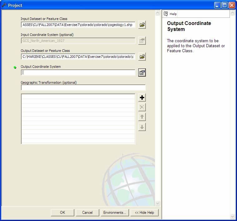
Geol 3050 – GIS for Geologists – Exercise 6

                 2. select geologic units for one time interval.
                 3. populate the new table by calculating the new value.

It is possible to select and reclassify several records at a time, as hand selecting this many records is extremely
tedious!

B1.      Adding a field to the table:

      5. Open the attribute table of the cogeology1_project.shp layer
      6. Examine the fields in the table.
      7. A quick way to examine the fields, is to sort them, either ascending or descending (or go back and
         forth):
         • Right click on the field name and select sort…(ascending\descending).
         • Do this for the text fields, and note that some of them are almost similar. How would you group in
             time intervals? Our goal is something similar as done by the CGS:
             See the Figure on Page 1

      8. Go to the upper left hand part of the of the table and click on the drop down Options menu (look for
         this button):

      9. Select Add Field…..
         (Close ArcCatalog if you get a warning message about another user!)

      10. Add the following parameters:
                 • Field Name: Time_Int                          Just a name.
                 • Field Type: Text                              Text vs Numeric Field.
                 • Field length: 30                              How many characters can be stored.

                                                             6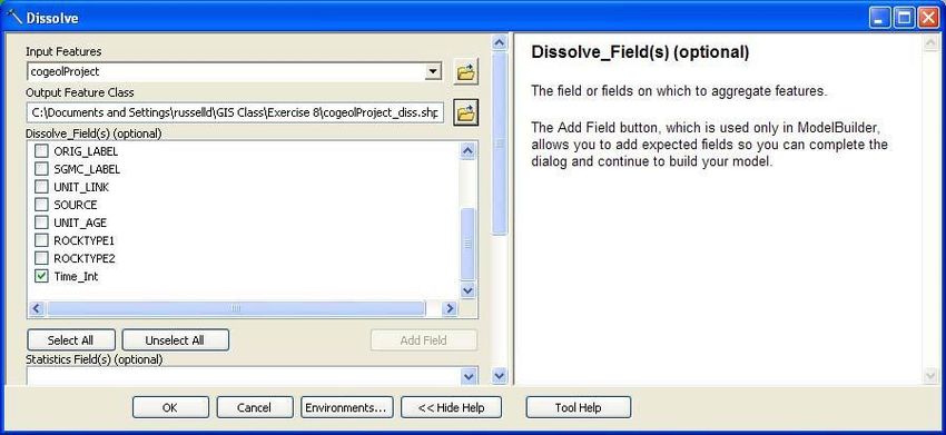
Geol 3050 – GIS for Geologists – Exercise 6

    11. Confirm that a new field has been added (right hand side, you might have to use the scroll bar at the
        bottom to see).

B2. Selecting records from the table:

    12. Go back to Options and select “Select by Attributes”

The Table Query window will now open. This will allow us to select certain records of the table. This will make
subsetting of our data into the following categories possible (We will use the categories used on the CGS
postcard):
            • Precambrian Rocks
            • Paleozoic Rocks
            • Mesozoic Rocks
            • Cenozoic Rocks:
            • Igneous Rocks
            • Sedimentary Rocks
            • Unconsolidated Deposits
    13. To select only the Precambrian Rocks, add the following formula in your table:

Notice the Logic (also called Boolean Algebra): by using the OR operator you are selecting the records in the
following way: if yes (statement = TRUE) then select the record, OR is there another statement to be checked,
is that statement true, then select that record too…. etc?

See Bolstad Chapter 9, page 303 for reference on Boolean logic.

HINTS:
For each query statement you need to DOUBLE CLICK on the name field [ORIG_LABEL]
For the = sign you only SINGLE click
For the name itself use ‘Name X’ or Click on the    Get Unique Values Button and DOUBLE Click the field
For the OR operator, Click the OR‐Button.

‐Copy/paste generally works but occasionally special marks (quotes, etc) don't always transfer over right.
Here's the formula: "ORIG_LABEL" = 'Yu' OR "ORIG_LABEL" = 'Yp' OR "ORIG_LABEL" = 'Yg' OR "ORIG_LABEL" =
'Yam' OR "ORIG_LABEL" = 'YXu' OR "ORIG_LABEL" = 'YXg' OR "ORIG_LABEL" = 'Xq' OR "ORIG_LABEL" = 'Xm' OR
"ORIG_LABEL" = 'Xg' OR "ORIG_LABEL" = 'Xfh' OR "ORIG_LABEL" = 'Xb' OR "ORIG_LABEL" = 'Wr'

                                                            7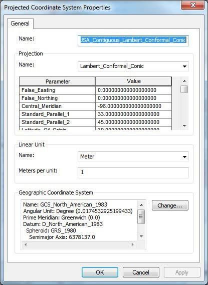
Geol 3050 – GIS for Geologists – Exercise 6

Verify your equation before running it! Then hit apply and close

    14. Verify your result by looking at the selected records on your map (they will show up in blue), but don’t
        click on the map, you might lose your selection!

B3. Calculating New Attribute Values

    15. Go to the top of your table, right click on the Time_Int column heading and select “Field Calculator”
    16. Fill exactly out (as shown here):

                                                            8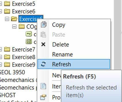
Geol 3050 – GIS for Geologists – Exercise 6

                “Precambrian”; Set the Field Type to String. Hit OK.

18. Your selected records in the table should say Precambrian now (as shown). The other records should have
remained empty.

This will be our trick to repopulate the table to “group” our records by age. We will have to repeat these steps,
but there are slightly faster ways:
Repeat previous steps B2 and B3 (see explanation on shortcuts below)

    17. Clear the selection first then clear expression in the “Select by attributes window” and repeat your
        steps for the other time intervals. You can actually do this in a quicker way as explained below:

                Tips:
                • Check your selections visually by looking at the map.

                                                            9
Geol 3050 – GIS for Geologists – Exercise 6
• Make sure you ONLY calculate the Time_Int field, and not any of the other text fields!!
• Typos are deadly!
• In case of problems you can “debug” your equation by cutting one statement out, and
then verify the rest of the equation.
Time groupings for each Geologic Unit
Example:
The Precambrian could actually be calculated quicker via the UNIT_AGE field (there should be 839 records
selected, and all the Time_Int Records )
Precambrian (2.8 bya – 544 my) “Precambrian”
Select the units in UNIT_AGE: Late Archean, Early Proterozoic, Middle Proterozoic and Early- Middle
Proterozoic
When you use the LIKE operator (instead of the = operator) with wildcards (charcters that can mean any
number or letter) to build a partial string search. The code language is called SQL, which is commonly use for
database queries.
If you are querying an ArcInfo coverage, shapefile, INFO table, dBASE table, ArcSDE data, ArcIMS feature class,
or ArcIMS image service sublayer:
'_' indicates one character.
‘X_’ means ‘X1’ Or ‘Xm’ but NOT ‘Xfh’
'%' indicates any number of characters.
‘X%’ means ‘X1’ Or ‘Xm’ but also ‘Xfh’
Shortcut for selecting:
"ORIG_LABEL" LIKE 'X%' OR "ORIG_LABEL" LIKE 'Y%' OR "ORIG_LABEL" = 'Wr'
This is happening: Select all records that start with an X, and also select all records that start with an Y, and
also select all records that are exactly “Wr”
These are all the rocks that are Precambrian X, Precambrian Y and Red Creek Quartzite
Now try these Paleozoic (544 – 253 my) “Paleozoic”
Try this shortcut to speed up the process (instead of an endless query, also documented in the HELP):
"ORIG_LABEL" LIKE 'MzPz' OR "ORIG_LABEL" LIKE 'Mm' OR "ORIG_LABEL" LIKE 'MD%' OR "ORIG_LABEL" LIKE
'MC%' OR "ORIG_LABEL" LIKE 'P%' OR "ORIG_LABEL" LIKE 'O%' OR "ORIG_LABEL" LIKE 'DO%' OR
"ORIG_LABEL" LIKE 'CA%' OR "ORIG_LABEL" LIKE '&%' OR "ORIG_LABEL" = '_am' OR "ORIG_LABEL" = '_l' OR
"ORIG_LABEL" = '_s' OR "ORIG_LABEL" = 'M_' OR "ORIG_LABEL" LIKE 'M_ml'
Mesozoic (253 – 65 my) “Mesozoic”
"ORIG_LABEL" LIKE 'TR%' OR "ORIG_LABEL" LIKE 'J%' OR "ORIG_LABEL" LIKE 'K%' OR "ORIG_LABEL" = 'Mz' OR
"ORIG_LABEL" LIKE '@%'
Cenozoic (0 – 65 my)
• "Cenozoic Unconsolidated"
10Geol 3050 – GIS for Geologists – Exercise 6
"ORIG_LABEL" LIKE 'Q%'
• "Cenozoic Igneous"
"ORIG_LABEL" = 'Taf' OR "ORIG_LABEL" LIKE 'Tbb%' OR "ORIG_LABEL" ='Tbr%' OR "ORIG_LABEL" LIKE
'Ti%' OR "ORIG_LABEL" = 'Tpl' OR "ORIG_LABEL" = 'Twm' OR "ORIG_LABEL" = 'Tv' OR "ORIG_LABEL" =
'Tui' OR "ORIG_LABEL" = 'Tmi'
• “Water”
Also select and classify all water bodies in the table, so there won’t be any “unclassified” holes in the
map.
"ORIG_LABEL" = 'H2O'
• "Cenozoic Sedimentary"
We saved this one for last because there are so many of them. Now we want to select everything
that has not been classified yet! Fill the field out in the following way: "Time_Int" = '' (2 single quotes)
***Note to change the FIELD Name here!!!!
!!!!! Check if indeed all values are starting with T (for Tertiary), and that there are no TR (Triassic) or Igneous
rocks classified! Or other rock from different time periods that were accidentally left out.
18. Deselect all records via the deselect button.
19. Now look at your map: nothing changed really since step 5…
20. To take advantage of your color scheme, change the symbology under Layer Properties. Under
Categories > Unique Values, set the classification field to [Time_Int] and ADD All Values. Assign the
following colors (according the USGS colorscheme in Appendix A):
• Precambrian light Grey
• Paleozoic Blue
• Mesozoic Green
• Cenozoic
• unconsolidated yellow
• sedimentary rocks brown
• igneous rocks red
• Water Lake Blue
11Geol 3050 – GIS for Geologists – Exercise 6
That was much easier than going through the entire list of different code_name values and setting them by
hand!
However, there is probably one thing obvious in your map: the map is made out of 7335 polygons
(i.e. records in the table!).
You can see this by looking at the boundaries between the polygons >>>>
12Geol 3050 – GIS for Geologists – Exercise 6
Part C. Geoprocessing operations
To really get rid of these internal boundaries (you can also take the outlines off the symbology) you can make
a new file with less polygons. ArcGIS has a Tool that is made to do this: the “Dissolve”‐function. It is part of a
series of spatial operations called “Geoprosessing functions”.
See Bolstad Chapter 9, page 313‐315 for reference.
21. Open ArcToolbox
22. Go to Data Management Tools > Generalization > Dissolve
24. This will create a new file “cogeology1_Project_Dissolve.shp” in your ArcMap project. Make sure you
select a “Dissolve Field” (i.e. Time_INT) and the HELP can be useful too. All polygons that have the
same value in the “Time_Int” field will be merged!
25. Symbolize your new layer via the Layer Properties.
26. Use the Import Symbology button to import the symbology.
27. Use the Import Symbology from another layer function to copy the symbology over (this is often a
13Geol 3050 – GIS for Geologists – Exercise 6
nice and quick way to set up symbology).
28. Look at the polygon boundaries, they should be gone (i.e. dissolved), even with the same
classification.
29. Open the attribute table of the new shapefile.
30. Check out the records in the table, how many polygons do you have now?
31. The result is very different.
The polygons are all grouped together, even if they are not next to each other. This is called a “multipart
polygon” structure. There is no way to see this in the file, except by selecting a record in the table, and look at
the result.
14Geol 3050 – GIS for Geologists – Exercise 6
32. Select one record in the table by clicking on the little arrow “>” sign.
33. Go to the Selection Menu > Zoom to Selected Features:
34. Notice that there are more than one individual polygons selected (because of the multipart feature),
but only one record in the table shows up!
15Geol 3050 – GIS for Geologists – Exercise 6
To Be Handed In!!!
• Make 2 screen dumps in a word document of your results on a single page:
1. The first should be of the cogeology1_project file turned on (with classification on the
Time_Int field).
2. The other will be of the cogeology1_project_Dissolve file turned on (with classification on
the Time_Int field) to illustrate the “dissolved” boundaries.
• SAVE your own shapefiles on a memory stick so you can use them for Exercise 7 and 8!!!!
• Save your ArcMap mxd project so you don’t have to redo the coloring for Exercise 7 and 8 (make sure
you use relative path names and save your project appropriately and just outside your exercise
folder). Copy everything (map .mxd + shapefiles) to your memory stick.
• Upload the file of your screenshots to the Canvas submission folder with your name in the document.
You can do this simply by adding your screenshots into a Word document, and then saving the file as a
PDF.
Summary:
• Queried and subsetted a file, based on the attribute table
• Added a field
• Calculated a field
• Used SQL query language
• Changed the symbology to match the assignment
• Used the Dissolve function to simplify the data.
16You can also read