Explaining the trends and variability in the United States tornado records using climate teleconnections and shifts in observational practices ...
←
→
Page content transcription
If your browser does not render page correctly, please read the page content below
www.nature.com/scientificreports
OPEN Explaining the trends
and variability in the United
States tornado records using
climate teleconnections and shifts
in observational practices
Niloufar Nouri1*, Naresh Devineni1,2*, Valerie Were2 & Reza Khanbilvardi1,2
The annual frequency of tornadoes during 1950–2018 across the major tornado-impacted states
were examined and modeled using anthropogenic and large-scale climate covariates in a hierarchical
Bayesian inference framework. Anthropogenic factors include increases in population density and
better detection systems since the mid-1990s. Large-scale climate variables include El Niño Southern
Oscillation (ENSO), Southern Oscillation Index (SOI), North Atlantic Oscillation (NAO), Pacific Decadal
Oscillation (PDO), Arctic Oscillation (AO), and Atlantic Multi-decadal Oscillation (AMO). The model
provides a robust way of estimating the response coefficients by considering pooling of information
across groups of states that belong to Tornado Alley, Dixie Alley, and Other States, thereby reducing
their uncertainty. The influence of the anthropogenic factors and the large-scale climate variables are
modeled in a nested framework to unravel secular trend from cyclical variability. Population density
explains the long-term trend in Dixie Alley. The step-increase induced due to the installation of the
Doppler Radar systems explains the long-term trend in Tornado Alley. NAO and the interplay between
NAO and ENSO explained the interannual to multi-decadal variability in Tornado Alley. PDO and AMO
are also contributing to this multi-time scale variability. SOI and AO explain the cyclical variability
in Dixie Alley. This improved understanding of the variability and trends in tornadoes should be of
immense value to public planners, businesses, and insurance-based risk management agencies.
Tornadoes are one of the most devastating, severe weather events in the United States (U.S.) that always pose
risks to human life and cause extensive property damage. Tornado outbreaks, defined as sequences of multiple
tornadoes closely spaced in time, lead to the most number of fatalities and rank routinely among severe weather
events that cause billion-dollar losses1. An average annual loss of $982 million is reported for U.S. tornado events
based on insurance catastrophe data from 1949–2006, which clearly indicates their destructive n ature2.
Modern logging of tornado reports in the U.S. has begun in the 1950s, and the reports grew even more in
the mid-1990s, mainly due to the increase in the detection of EF0–EF1 category tornadoes (weak tornadoes)
after the installation of the NEXRAD Doppler radar s ystem3–10. Other factors, such as better documentation,
more media coverage, rise in the population, and storm chasing also contributed to this increased detection rate.
Recent studies show that this secular trend (i.e., the long-term trend that is not due to seasonality) in the annual
frequency of tornadoes has also been varying spatially. See, for example, Gensini and Brooks11 who showed that
the temporal trends since 1979 have a significant spatial variability, and Moore12, who found that the number
of tornadoes per year increased in the southeast U.S. and has decreased in the Great Plains and the mid-west
regions. Studies by Farney and Dixon13 and Agee et al.6 show similar results.
Figure 1 presents the confirmation of trends in the annual frequency of tornadoes in 28 major tornado-
impacted states in the U.S. Statistically significant secular trends (as estimated using the Mann Kendall Sen
Slope14) are found in 26 states. Evidently, there also seems to be a step-change in many of these states since
the 1990s, along with signs of cyclical trends in others (for example, Texas, South Dakota, and Florida). The
inter-annual variability is also prominent and seems to have increased in recent decades. That the inter-annual
1
Department of Civil Engineering, The City University of New York (City College), New York, NY 10031,
USA. 2NOAA/Center for Earth System Sciences and Remote Sensing Technologies (CESSRST), The City University
of New York (City College), New York, NY 10031, USA. *email: nnouri@ccny.cuny.edu; ndevineni@ccny.cuny.edu
Scientific Reports | (2021) 11:1741 | https://doi.org/10.1038/s41598-021-81143-5 1
Vol.:(0123456789)
www.nature.com/scientificreports/
Figure 1. Annual number of tornado incidence in 28 major tornado-impacted states in the U.S. during
1950–2018. The blue line is locally-weighted polynomial fit20 using a smoothing span of 0.5. For each state,
Mann–Kendall trend test is performed and the p-value of the test along with Sen’s slope or the rate of change is
presented.
Scientific Reports | (2021) 11:1741 | https://doi.org/10.1038/s41598-021-81143-5 2
Vol:.(1234567890)
www.nature.com/scientificreports/
Figure 2. (a,b,e,f) represents the time series plots for the scores of the first four principal components. The
pink line is the locally weighted smoothing line with span of 0.1. (c,d,g,h) is the wavelet power spectrum of the
corresponding score. Higher wavelet power during a specific time shows notable frequencies in tornado activity.
The areas with solid black line represent significant wavelet power at the 90% confidence interval. (Wavelet plots
are created in R version 3.5.2 using biwavelet package26, https://CRAN.R-project.org/package=biwavelet).
variability in tornado counts relates measurably to El-Nino Southern Oscillation (ENSO), a large-scale climate
teleconnection feature is not unknown. See, for instance, Cook and S chaefer15, Lee et al.16, Marzban et al.17, and
Allen et al.18, among others. A recent investigation of the tornado activity in the southeast U.S. region noted an
association with the North Atlantic Oscillation (NAO) in addition to ENSO and regional sea surface temperature
anomalous patterns19.
A more in-depth examination that we conducted using robust principal components analysis and wavelet
transformation to decipher the hidden structures in the time series of the tornados’ annual frequency across the
28 major tornado-impacted states revealed systematic low-frequency oscillations beyond the inter-annual time
scale. We show this in Fig. 2. The high-dimensional annual tornado frequency data (69 years of counts data for
the 28 major tornado-impacted states) was first reduced to its dominant modes using robust principal compo-
nents analysis21 (rPCA). The first four dominant modes (principal components or scores) explained up to 93%
of the original data variance with the first mode capturing the secular trend in the data as a result of increased
tornado detection. The other modes exhibited cyclical variability. Wavelet t ransformation22–25 of these princi-
pal components unveiled oscillatory features at the interannual to multidecadal time scales with much lower
Scientific Reports | (2021) 11:1741 | https://doi.org/10.1038/s41598-021-81143-5 3
Vol.:(0123456789)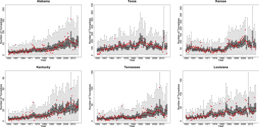
www.nature.com/scientificreports/
frequency signals in the third and the fourth modes. For example, the wavelet analysis of the first three principal
components showed significant wavelet power (at the 90 percent confidence interval) occurring in period band of
2–5 years, which reveals notable variability in the data with a frequency of 2–5 years. This typically corresponds
to low-frequency climate variability. The significant period band of 2–5 years occurred in mid 1960s and during
2000–2010 in the first PC, while in the second PC, the periodic activity was significant during 1970 to mid-80s,
mid 1990s and 2000–2012. The third principal component also reveals similar period band which was notable in
early 1960s and 2005–2015. The power spectrum plot of the third PC (2-g) showed a significant wavelet power
at a period band of 5–10 years during mid-1980s to mid-1990s, which suggests decadal oscillatory behavior.
These preliminary inquiries and experiments prompted us to devise a comprehensive modeling approach
to infer the key explanatory factors of the annual frequency of tornadoes across the major tornado-impacted
states in the U.S. There is evidence of secular trend and cyclical variability, and this might vary spatially. Hence,
there is a need to understand the effects of possible anthropogenic factors and large-scale climate teleconnec-
tions separately.
Anthropogenic factors such as the rise in population and the installation of better detection systems may have
led to a monotonic increase or a step-change in the frequency of tornadoes. Hence, to explain the secular trend,
we choose two indicators—the annual population density data (PD) for each state and a binary Doppler Radar
Indicator (DRI) with zero from 1950–1990 and switches to 1 from 1991–2018—to factor in the installation of the
NEXRAD Doppler radar system in the early 1990s. Large-scale climate oscillations may control the interannual
to multidecadal variability seen in the data. Hence, to explain the cyclical trend, we factored in a suite of annual
climate indices—El Niño/Southern Oscillation (ENSO)—through the Nino3.4 index, Southern Oscillation Index
(SOI), North Atlantic Oscillation (NAO), Pacific Decadal Oscillation (PDO), Arctic Oscillation (AO) and Atlantic
Multi-decadal Oscillation (AMO). We conducted a wavelet coherence analysis27–29 between the first four principal
components described in Fig. 2 and these climate indices for additional validation of their selection. Evident
joint variability is seen in the coherence plots (see Figure S2 in the supplemental material), indicating that the
low-frequency oscillation of climate could drive part of the variability in the tornadoes’ annual frequency. As
mentioned before, these anthropogenic and climate effects can vary in space. Still, there is a possibility of some
commonality in the impacts over specific regions, such as the Tornado Alley, Dixie Alley, etc.3,30,31.
These conditions inspired us to build nested models using a hierarchical Bayesian inference framework,
which not only allows for a full uncertainty quantification but also its reduction by pooling information across
appropriate classification of states. The hierarchical framework provides an elegant means of propagating the
parameter uncertainty through appropriate conditional distributions. Further, noting that multiple climate and
anthropogenic covariates influence tornadoes across a region (Tornado Alley, Dixie Alley, etc.) similarly, the hier-
archical model provides pooling of this common information. This type of pooling reduces the equivalent number
of independent parameters, resulting in lower uncertainty in parameter estimates. The models are explained
in detail in the Methods section. Using this holistic modeling framework, for the first time, we explained the
factors governing secular trends and cyclical variability in the annual frequency of tornadoes across the major
tornado-impacted states in the U.S. The relative contribution of the anthropogenic and climate factors and their
primary influence regions are discussed.
Results
Explaining the variance. Figure 3 presents the spatial distribution of the explained variance from the
nested models (M1 and M 2—see the Methods section for a description of these models). We first show the state-
level R2 of M
1, the model that uses PD and DRI as the anthropogenic covariates to understand their influence
in producing the secular trend. The state-level R2 of model M2 that uses these two anthropogenic covariates as
well as the climate covariates (SOI, NAO, the interaction between Nino3.4 and NAO, PDO, AMO, and AO) is
shown next. The difference in the R2 between the two models is also presented. This difference map measures the
additional explanation that the climate covariates provide in each state. Table S2 in the Supplemental Material
provides the numerical details for each state.
The two anthropogenic covariates explained 17%, 28%, and 19% of the variance in the annual tornado fre-
quency on average across Tornado Alley, Dixie Alley, and Other States, respectively. Greater than 30% variance
in Kansas, Alabama, Mississippi, Kentucky, and Minnesota was explained by these covariates alone. Climate
covariates brought additional explanation in the order of 15%, 11%, and 5% on average in the three groups,
respectively raising their total average explained variance to 32%, 40%, and 24%. The largest increments in the
variance explained were in Texas (29%), South Dakota (22%), and Florida (20%), indicating that climate plays a
significant role in modulating the annual tornado frequency in these states. Based on the significant covariates
from the model, we can infer that in Texas, all except SOI play a role, in South Dakota, it is primarily from NAO
and AMO, and in Florida, NAO, AMO, PDO, and AO feature as the control variables. Similar inferences can be
drawn for other states using Table S3, which shows the p-values for all the response coefficients.
Overall, the anthropogenic and the climate covariates explained more than 40% variability in the annual tor-
nado frequency in eight states, and more than 30% variability in 11 states. For these states, and Texas (explained
variance = 33%), Tennessee (explained variance = 47%), and Louisiana (explained variance = 41%), we present the
posterior distribution of the annual tornado frequency in Fig. 4. They are presented as a time series composed
of boxplots instead of single points because the tornado counts for each year are estimates of the posterior dis-
tribution for those years. The boxplots depict those posterior distributions graphically. The record of observed
tornado counts data are also shown (red circles) along with an 11-year low-pass filter to visualize the general
trend in the data. Secular trend dominated in Alabama (R2 = 43% from M1 vs. 54% from M 2), Kentucky (R2 = 54%
from M1 vs. 60% from M2), and Kansas (R2 = 40% from M1 vs. 54% from M2). Climate trend dominated in Texas
(R2 = 5% from M1 vs. 33% from M2). In Tennessee (R2 = 28% from M1 vs. 47% from M2) and Louisiana (R2 = 25%
Scientific Reports | (2021) 11:1741 | https://doi.org/10.1038/s41598-021-81143-5 4
Vol:.(1234567890)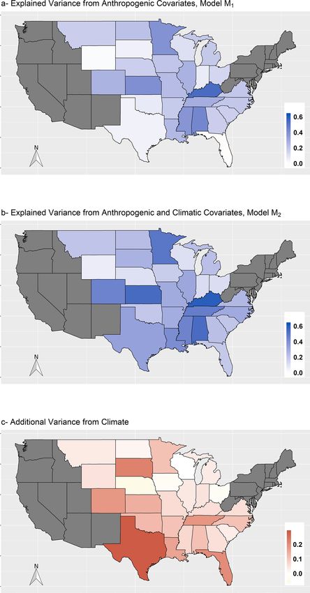
www.nature.com/scientificreports/
Figure 3. Spatial distribution of the explained variance from the nested models
( M1 and M2). The explained
y )2
(y −
variance, i.e., R2, is calculated based on sum of squared residuals, Ri2 = 1 − it −it 2 , where yit and
yit are the
(yit − y i ) −
observed and the predicted posterior median of the tornado counts in year t and state i, and y i is the mean of
the observational data during the entire period. (Maps are created in R version 3.5.2 using the ggplot2 p ackage32,
https://CRAN.R-project.org/package=ggplot2).
from M1 vs. 41% from M 2), there was evidence of a mixture of these effects. Across all the states, the hierarchical
Bayesian model did well in capturing the secular and cyclical trends while producing the uncertainty intervals.
Texas and Kansas were particularly interesting cases due to an existence of low-frequency oscillation and
step change. Texas showed a multidecadal variability signal, which was represented well in the model’s posterior
distribution. Kansas showed a step increase in the annual tornado counts since the 1990s, which was followed
by an increase until the early 2000s and a decrease in tornados recently. In this case, too, the posterior distribu-
tion captured the three significant changes, thus indicating the model’s ability to predict changes based on the
anthropogenic and the climate covariates.
To evaluate the posterior distributions of the annual tornado counts, we also verified the coverage rates within
the credible intervals and conducted posterior predictive checks. These results are presented in Table S2 of the
Supplemental Material. The posterior predictive distribution of the annual tornado counts was assessed by exam-
ining the model’s ability to cover the observed counts (coverage rate) within a 95% credible interval33. For each
state, we computed the coverage rate as the percent number of observations that are inside the 2.5th and 97.5th
percentile of the posterior distribution. The average across each of the Alleys was approximately 95%, indicating
Scientific Reports | (2021) 11:1741 | https://doi.org/10.1038/s41598-021-81143-5 5
Vol.:(0123456789)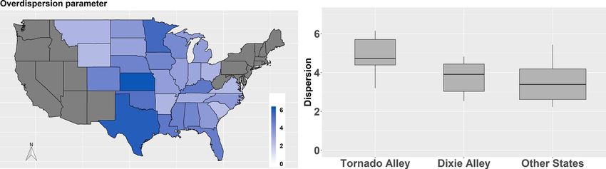
www.nature.com/scientificreports/
Figure 4. Boxplot of posterior distribution of tornado counts in Alabama, Texas, Kansas, Kentucky, Tennessee
and Louisiana. The median of posterior distribution in a state can be referred to the estimated annual tornado
counts in that state. The red circles and red line represent annual records of observed tornado counts along with
an 11-year low-pass filter to visualize observed trend.
Figure 5. Map of median overdispersion parameter from the negative binomial distribution along with its
group-level distribution in Tornado Alley, Dixie Alley and Other States. (The map is created in R version 3.5.2
ackage32, https://CRAN.R-project.org/package=ggplot2).
using the ggplot2 p
the robustness of the fitted Bayesian models. Following Gelman et al.34, we also computed the Bayesian p-value
for two test quantities—the 10th percentile of the data (y[10]) and the 90th percentile of the data (y[90]). Bayesian
p-value is defined as the probability that the replicated data (yrep) could be more extreme than the observed data
(y) as measured by the test quantities, i.e., Pr(T(yrep , θ ) ≥ T(y, θ)|y). The mean p-value for each of the states is
presented in Table S2. The tail area probabilities in all the cases were within 0.05 and 0.95, indicating that the
model can replicate the observed data well. These verifications confirmed our confidence in interpreting the
results and our inference of the response parameters in the model.
Next, we present overdispersion in the data as modeled using r, the overdispersion parameter (see “Methods”
section for details). Figure 5(left-panel) shows the spatial distribution of the median of the posterior distribution
of r. An overdispersion factor that is close to 1 indicates that the data resembles a Poisson distribution with an
expected value equal to the variance. Higher values of r indicate that the variance is greater than the mean, or
that there is more variance (relative to the mean) in the annual tornado counts—a fat tail distribution. All the 28
states had an overdispersion factor that is greater than 2. Kansas, Texas, Minnesota, and Oklahoma were among
the states that had a high dispersion factor over 5. We also found that the overdispersion parameter is different
in the three groups—Tornado Alley, Dixie Alley, and Other States. Figure 5(right-panel) shows the results of the
dispersion parameters for each group as boxplots. The states in Tornado Alley had relatively higher dispersion
factors compared to those in Dixie Alley and Other States. The median dispersion factor in the Tornado Alley
was 4.7, whereas it was 3.9 and 3.4 in the Dixie Alley and Other States, respectively. Other States had more spread
compared to the states in Dixie Alley with some dispersion factors exceeding 5. It was also interesting to note
that among the 13 states with a dispersion factor exceeding 4, the median amount of variance we could explain
is at least 40% indicating the model’s ability to predict fat-tail events well.
Scientific Reports | (2021) 11:1741 | https://doi.org/10.1038/s41598-021-81143-5 6
Vol:.(1234567890)www.nature.com/scientificreports/
Figure 6. (a–h) maps of the regression coefficients expressed as percentage change in the expected annual
tornado counts per unit change in the covariate (for figure a, population density, we measure change per
an increase of 10 people/mi2); (i) posterior distributions of the mean of the regression coefficients from the
hierarchical level as boxplots per the three state-groups. Color scheme in the maps indicates the direction (blue
for positive response and orange for negative response); thick boundaries shows the states that have a significant
positive or negative association of annual tornado frequency with the corresponding covariate. (Maps are
created in R version 3.5.2 using the ggplot2 package32, https://CRAN.R-project.org/package=ggplot2).
Inference of the significant predictors. In Fig. 6, we present
j
the state-level significant covariates
(Fig. 6a–h, based on the inference of the regression coefficients βi[k]) and their group-level (regional) effects
(Fig. 6i, based on the inference of µkβ j ). The color scheme in Fig. 6a–h indicates the direction (blue for positive
response and orange for negative response) and the strength of association expressed as percentage change in the
expected annual tornado counts per unit change in the covariate. A thicker boundary shows states that have
j j
Pr(βi[k] > 0) > 0.95 or Pr(βi[k] > 0) < 0.05. These are the states that have a significant positive or negative associa-
tion of annual tornado frequency with the corresponding covariate. Figure 6i presents the posterior distributions
of µkβ j (i.e., the mean of the regression coefficients from the hierarchical level) as boxplots per the three state-
groups. Full numerical details are presented in Table S3 in the supplemental material.
Population density was a significant predictor in all of the Dixie Alley states and much of the Other States
(Fig. 6a). As expected, it had a positive effect—an increase in the population density is associated with an increase
in the rate of annual tornadoes, thus best explaining the secular trend. In the Dixie Alley states, there was between
Scientific Reports | (2021) 11:1741 | https://doi.org/10.1038/s41598-021-81143-5 7
Vol.:(0123456789)www.nature.com/scientificreports/
6–57% increase in the rate of annual tornadoes per additional ten people/mi2, the largest rate being in Mississippi
(57%). In other states, the rate of increase in annual tornadoes ranged from 2% (in Florida) to 27% (in Kentucky)
per ten people/mi2. Except for Colorado, population density was not a significant predictor in the Tornado Alley
population
states. The posterior distribution of the regional coefficient (µβ , the hierarchical level mean for betas-
population) clearly indicates this effect. The regional mean is an indication of the average impact of population
density in the respective state-groups. Dixie Alley states and Other States have a positive mean coefficient at a rate
of increase of 28% and 12% per ten people/mi2, while the Tornado Alley states have a mean in the range of zero.
While the population density was a significant predictor in the Dixie Alley, the Doppler Radar Indicator was
a significant predictor in the Tornado Alley and nine states in the Other States category (Fig. 6b). These were the
states where step-change due to the Doppler Radars installation in the 1990s best explains the secular trend. In
the Tornado Alley, there has been a 34–69% increase in the rate of annual tornadoes since the 1990s. Based on
the mean of the regression coefficients, we can deduce that regionally, there has been a 46% increase in the rate
of annual tornadoes (since the 1990s) in Tornado Alley. This increase in the rate is 40% in Other States.
The next six panels in Fig. 6 displays the coefficients for the climate covariates. The Southern Oscillation
Index (SOI) was a significant predictor in Alabama and Tennessee in Dixie Alley and several states from the
Other States group, but not significant in Tornado Alley. The boxplot of the mean of the regression coefficients
showing the regional effect further reinforces this inference. However, the interaction term between ENSO and
NAO, as treated by Nino3.4*NAO, was significant in four states in Tornado Alley (Colorado, Kansas, Oklahoma,
and Texas), i.e. ENSO had an impact on the Tornado Alley during NAO events. The posterior distribution
µβ − ENSO.NAO also underlines this finding. On the other hand, NAO had a negative effect, mainly in Tornado
Alley and Other States, not in Dixie Alley.
Previous studies on tornado variability also identified ENSO and NAO as significant influence variables. For
instance, Cook and Schaefer studied the impact of ENSO phases on the location and strength of U.S. tornado
outbreaks from 1950–200315. Based on historical observations, they suggested that sea surface temperature
oscillation in the tropical Pacific has different effects on the likelihood of tornado outbreaks depending on the
geographic region. El Niño episodes usually limit tornado outbreaks in the Gulf Coast states, including central
Florida. At the same time, La Niña affects a larger zone stretching from southeast Texas northward to Illinois,
Indiana, and Michigan. Lee and Wittenberg studied springtime ENSO evolution and its potential links to regional
tornado outbreaks using records between 1950 and 2 01416. Their findings showed that in a resurgent La Niña,
the probability of a tornado outbreak significantly increased in the Ohio Valley and the upper Midwest. On the
other hand, when a two-year La Niña transitions to an El Niño, the risk of a tornado outbreak rises in Kansas
and Oklahoma. Marzban and Schafer also examined the correlation between regional tornado activity and sea
surface temperature (SST) in four zones in the tropical Pacific O cean17. They found that the strength of correla-
tion in different U.S. regions varied depending on the selected zone in the Pacific Ocean. However, their findings
generally identified a strong correlation between cool SST in the central tropical Pacific (La Niña episode) and
tornadic activity in an area stretching from Illinois to the Atlantic Coast, and Kentucky to Canada. Allen et al.
showed that ENSO influences tornado activity by altering the favorable large-scale environmental conditions
such as vertical wind shear and thermodynamic potential energy. Their study revealed that ENSO affects spring
and winter tornado occurrences by modulating the position of the jet stream over North A merica18. The study
suggested that La Niña causes the atmospheric jet stream to move southeastward, which favors tornado formation
in central states due to the temperature gradient. Conversely, El Niño episodes reduce the chances of tornados
occurring in the central U.S. due to the weakening of surface winds that typically carry warm and humid air
from the Gulf of Mexico. Lee et al.35 also discussed that the decay or development of ENSO (Trans-Niño) could
led to a pattern of cool temperatures in the central Pacific and warm sea surface temperatures over the eastern
tropical Pacific which produced more conducive for spring tornado outbreaks. Cook et al.36 also investigated the
relationship between sea surface temperature in Nino3.4 region and U.S. tornado outbreaks (in terms of counts
and destructive potential) during winter and early spring. Their results showed that La Niña phases are consist-
ently associated with more frequent and stronger tornadoes compared to El Niño conditions. They discussed
that this tornado variability is related to the strength and location of subtropical jet during each outbreak and
the positions of surface cyclones and low-level jet streams.
In a very recent study, M oore37 explored the relationship between seasonal tornado frequency (from 1953
to 2016) and El Niño/Southern Oscillation (ENSO) for multiple U.S. regions. They also examined the spatial
dependence of the Tornado Frequency–ENSO relationship and showed that winter and spring tornadoes in
the Southeast and Midwest regions were related to ENSO, and the relationship was stronger in winter than
in spring in both regions. Mean and median tornado frequencies of the La Nina seasons were notably greater
than the other phases’ mean and median. They found a significant negative correlation between winter tornado
frequency and ONI (anomalies of 3-month running means of sea surface temperature in the Niño 3.4 region)
in Southeast and Midwest.
The study by Molina et al.38 showed that El Niño, La Niña, and positive phase of SST anomalies in Gulf of
Mexico are linked to increased winter tornadoes; El Niño contributed to increased activity in the Southeast U.S.,
and La Niña increases tornado activity in Midwest and Midsouth. They also reported that tornado favorable
conditions were significantly related to anomalously warm and cool SSTs at the Gulf of Mexico. Lepore et al.39
investigated the modulation of U.S. convective storms by El Niño–Southern Oscillation and showed that spring
tornado activity could be predicted using December-February NINO 3.4 values because ENSO is usually per-
sistent from winter to spring.
The study by Elsner et al.19 reported an association between the NAO and tornado activity in the southeast U.S.
The findings of this study showed that a positive phase of the NAO (lower than normal pressures over Greenland
and higher than normal pressures over the Atlantic) is linked to a lower chance of tornadoes developing across
southeastern states, Arkansas, Missouri, and Kentucky. S pencer40, a former NASA climate scientist looked into
Scientific Reports | (2021) 11:1741 | https://doi.org/10.1038/s41598-021-81143-5 8
Vol:.(1234567890)www.nature.com/scientificreports/
the correlations between the Pacific Decadal Oscillation (PDO) and strong tornadoes, EF3 to EF5. His finding
showed that the positive phases of PDO, which was dominant from the mid-1970s until 2005, is associated with
fewer tornadoes in the U.S.
The study by Muñoz and Enfield41 presented the relation of Intra-Americas low-level jet (IA-LLJ) variability
with Atlantic and Pacific climate teleconnections. They calculated Spearman correlations between tornados
and the following: NAO, Pacific/North American teleconnection (PNA), Pacific decadal oscillation (PDO), and
Niño3.4. The highest correlation achieved between March PNA and March (April) tornado activity is − 0.46
(− 0.33). Their findings revealed that an enhancement of the intra-Americas low-level jet stream during the cold
phase of Niño3.4, was linked to an increased occurrence of tornadoes in the east of the Mississippi River. They
also reported a connection between negative phase of the PNA pattern during spring and intensification of the
IA-LLJ, which could provide greater moisture to the Mississippi and Ohio River basins and lead to increased
tornadic activity.
Elsner and Widen42 used a Bayesian model to predict seasonal tornado records within a region that stretches
across the central Great Plains from northern Texas to central Nebraska. The authors assumed that tornado
counts follow a negative binomial distribution and used the sea surface temperatures (SST) over the western
Caribbean Sea and Gulf of Alaska during February as predictors. A trend term was also included to account for
improvements in tornado reporting over time. The study showed that SST from both regions during February
had a significant link to springtime tornado activity across the central Great Plains. There was a 51% and 15%
increase in tornado counts per degree Celsius increase in SST of western Caribbean and Gulf of Alaska, respec-
tively. The study showed that the SST covariates explained 11% of the out-of-sample variability in the observed
F1–F5 tornado reports. The authors concluded that adding a pre-season covariate for the El Niño, PDO and
NAO does not improve their model. Guo and W ang43 studied how temporal trends of EF1+ tornadoes varied
across the 48 U.S. states during 1950–2013. Their study showed that The Great Plains (including Nebraska and
Texas) and Southeast (including Kentucky, Virginia, Tennessee, North Carolina, South Carolina, Alabama, and
Georgia) are contributing to the continental‐scale increase in tornado temporal variability.
While our finding regarding ENSO and NAO corroborate previous conclusions based on regional studies,
we provided comprehensive state-level summaries through these results using a holistic model. Besides, beyond
the findings regarding ENSO and NAO, we also found that PDO events have a significant positive effect in Colo-
rado and Texas in the Tornado Alley and all states in the Other States, but do not affect Dixie Alley. The boxplots
of the µβ in Fig. 6i is further evidence of this regional effect. AMO, too, modulates the tornado variability in
several states in Tornado Alley and Other States, but not Dixie Alley. Similar to NAO, it had a negative effect on
the states it influences. Finally, we find that AO modulated the variability in almost all the states and had a posi-
tive effect. The positive AO phase enhances the rate of tornadoes in these states. A positive AO phase typically
creates a warmer than normal winter in the U.S. through the polar vortex a ctivity44 that keeps colder front far
north. Warm winters are in turn related to above normal tornado activity. Childs et al.45, through a correlation
analysis, have previously shown that positive AO phase can be related to enhanced winter season (November
to February) tornado activity.
Recognizing that there will be uncertainty in estimating model coefficients due to uncertainties in the input
data, especially the choice of where the binary indicator changes from 0 to 1, we also conducted additional
experiments to verify the model sensitivity to changes in when this binary indicator shift happens. The model
estimation is done for all potential start years from 1991 to 1997. From each of these models, we present in
Figure S3, the distributions of the mean of the regression coefficients (µkβ j ) to verify whether the regional effect
changes with change in the input binary variable. We find that the distributions of the mean regression coeffi-
cients for the anthropogenic and the climate covariates are similar. While these verification experiments indicate
that the model results are robust to changes in inputs, we urge caution in interpreting the coefficients for specific
states. We recommend an approach where the model can be updated if new data is available regarding when the
Doppler Radar system installation happened in particular states.
Discussion
Whether the frequency in U.S. tornadoes has changed in the last century had been a tricky question to answer
reliably given the changes in the classification of the tornadoes and reporting practices4,46–49, and significant and
possibly increasing interannual variability inherent in the data5,50,51. Verbout et al.9 attempted to address this
question by fitting linear trend models on individual categories (F/EF scales) in the data for the aggregated counts
across the U.S. Others, based on regional analyses, showed that these trends could vary spatially6,11,13. However,
to our knowledge, a comprehensive assessment of explaining trends and variability across the U.S. by separating
secular trends from cyclical variability has not been conducted previously, and hence motivated us to embark
on this research of classifying the climatological trends across 28 major tornado-impacted states in the U.S.
In general, this is a high-dimensional problem that offers interesting opportunities since the trends and
climate responses have local (state-level) as well as regional (alley-level) effects. A hierarchical Bayesian model
with partial pooling was an excellent fit to seamlessly capture these at-state and regional effects. Partial pool-
ing through a hierarchical model also offers a reduction in the uncertainty of the trend/response coefficients.
Hierarchical Bayesian models are being used more commonly in applications related to predictions and data
description, especially for multivariable problems where the investigator needs to learn something about the
group and individual dynamics. Recently, Potvin et al.52 used such Bayesian hierarchical modeling framework
to estimate tornado reporting rates and expected tornado counts over the central U.S. between 1975–2016 while
also addressing spatial non-uniqueness issues. Our study builds on this work and provides an application for
seamless estimation of secular and cyclical trends in the annual frequency of tornados across the U.S.
Scientific Reports | (2021) 11:1741 | https://doi.org/10.1038/s41598-021-81143-5 9
Vol.:(0123456789)www.nature.com/scientificreports/
In our models, we attributed the state-level secular trend to two anthropogenic covariates (population density
and Doppler radar installation indicator). The regional secular trend was then estimated with the hierarchical
model through the pooling of information within the alleys. We attributed the state-level cyclical variability to six
climate covariates (SOI, NAO, PDO, AMO, AO, and an interplay term between ENSO and NAO). The common
climate response in each of the three alleys was estimated in the partial pooling hierarchical level. By separating
the covariates and looking at their difference in the variance explained, we described the effect of large-scale
climate in modulating the variability on top of the anthropogenic factors.
We found that, in essence, population density explains the secular trend in Dixie Alley. In contrast, the step-
change induced due to Doppler Indicator explains the secular trend in Tornado Alley. The states in the Other
States group were affected by a combination of both factors. The secular trend in these states is partly due to
population increases and partly due to Doppler radar installation. NAO and the interplay between NAO and
ENSO explained the inter-annual to multi-decadal variability in Tornado Alley. Further, we found that PDO and
AMO are also contributing to this multi-time scale variability. SOI and AO can explain the variability in Dixie
Alley. In the rest of the Other States, interannual to multi-decadal variability was modulated by all the climate
covariates, except the interaction term.
These findings regarding PDO, AMO, and AO on the annual frequency of state-level tornadoes across the
U.S. are presented here for the first time, and provoke thinking and systematic investigation as to how such low-
frequency oscillations may work in modulating the regional variability of tornadoes, and whether the underlying
climate processes can suggest, at least qualitatively, that the inference we find here can be explained. Extending
this inference model into a seasonal forecast setting using pre-season climate v ariables53 would be of interest too.
Such prognostic information is of value to public planners, businesses, and insurance-based risk management
agencies53. The more we can understand and predict tornado prevalence and occurrence, the more resilience
we build to these catastrophic events.
Methods
Data. Tornados. Historical tornado records were retrieved from the United States (U.S.) Storm Prediction
Center (SPC). The SPC’s tornado data represents the most reliable accounting of tornado occurrence available
over the U.S.11,42 This dataset is collected and compiled from National Weather Service (NWS) Storm Data pub-
lications and reviewed by the U.S. National Climate Data Center9,50,54. The dataset includes information about
the date and time, location, path, intensity (Fujita or enhanced Fujita (EF) scale), property losses, crop damages,
fatalities, and injuries records on all tornado incidents in the U.S. from 1950 till date. The tornado database can
be accessed online at https://www.spc.noaa.gov/wcm/. 55 Since the records of tornado occurrence in this dataset
is primarily based on eyewitness and reports of storm damages, there might be spatial biases in the data due to
the varying population density56.
Further, It is widely believed that the number of actual tornado occurrences is greater than the number
of reported values, especially before the deployment of the Weather Surveillance Radar-1988 Doppler (WSR-
88D)4,15,57,58. The primary sources of error are the undetected tornadoes and the lack of consistency in reporting
standards. Due to the short-lived and unpredictable nature of tornadoes, they are more likely to be documented
if people observe them directly or leave some visual evidence. Accordingly, tornado detection in less populated
areas or regions with inadequate communication facilities is challenging. Given that most tornado reports rely on
human observations and damage assessments, a region’s population has a critical influence on reporting. Normal-
izing tornado statistics for population bias has been of interest, and several studies have investigated the effect of
population change on tornado frequency reports. S nider59 looked into the tornado frequency in urban and rural
Michigan between 1950–1973 and found a positive correlation between population density and the probability
of a tornado being observed and recorded. A study in 1 98160 estimated that it is extremely hard for a tornado to
go unobserved when population density is above 1.5 people per km2. Evidence suggests that F2–F5 tornadoes
(where F stands for “Fujita scale”) are more likely to be reported due to their greater intensity and longer dura-
tion than weaker tornadoes F0–F1. This supports the idea that reports of larger tornadoes are less affected by
population density, and the inconsistency/disparity in tornado reports is primarily for F0-F1 c ategories57,61.
The impact of human error on the spatiotemporal variabilities of tornado reports is more emphasized before
improvements to the weather radar network. Introduction of the Operational Implement of WSR-88D radars is a
key factor contributing to more tornadoes reported since 1 99062. Since its introduction, the number of tornado-
related deaths and personal injuries has decreased by 45 percent and 40 percent, r espectively63. The emergence
of cellular phones, local emergency management offices, and rapid information spread through local media are
among other non-meteorological factors contributing to more tornado reports62. Less strong tornadoes remain
undocumented in sparsely populated regions or areas with insufficient communication i nfrastructure49.
In this study, we considered the annual tornado frequency during 1950–2018 of 28 major tornado-impacted
states located in South, Southeast, Ohio Valley, Upper Midwest, and Northern Rockies. Six of these 28 states
(Texas, Oklahoma, Kansas, Colorado, Nebraska, and South Dakota) are previously classified as the states that
belong to the significant Tornado Alley31,64. Another six states (Arkansas, Louisiana, Mississippi, Tennessee,
Alabama and Georgia) are classified as Dixie Alley states3,30. A complete list of the 28 states along with their
classification into Tornado Alley states, Dixie Alley states, or Other States is presented in Table S1 of the supple-
mental material. In Figure S1 of the supplemental material, we show the spatial distribution of all the tornadoes
during 1950–2018.
Population density. Population data for these 28 states were obtained from the U.S. Census Bureau, Population
Division. Population counts are collected from the census, which occurs every ten years. Using current data of
births, deaths, and migration, the population estimate program (PEP) computes population changes from the
Scientific Reports | (2021) 11:1741 | https://doi.org/10.1038/s41598-021-81143-5 10
Vol:.(1234567890)www.nature.com/scientificreports/
latest decennial census, and calculates and updates population count every year. Every annual issuance of popu-
lation estimates are utilized to revise the entire time series of estimates from July 1, the recent census day of the
current year. Full details of the applied methods are found online at https://www2.census.gov/programs-surveys/
popest/technical-documentation/methodology/2010-2018/2018-natstcopr-meth.pdf. 65 Population density was
computed by dividing the population by the state’s area and expressing the values in persons per square miles.
Large‑scale climate. We used El Niño/Southern Oscillation (ENSO)-Nino3.4, Southern Oscillation Index
(SOI), Arctic Oscillation (AO), Atlantic Multi-decadal Oscillation (AMO), Pacific Decadal Oscillation (PDO)
and North Atlantic Oscillation (NAO) annual indices to quantify the effect of large-scale climate on the inter-
annual variability of tornadoes. Some of these large-scale climate variables were previously found to be signifi-
cant in explaining the variability in t ornadoes15–19. We retrieved the monthly time series for these indices from
the National Oceanic and Atmospheric Administration’s (NOAA’s) National Centers for Environmental Predic-
tion (NCEP). Annually averaged indices are used in the model. Several recent studies explored the connection
between tornado activity and other climate oscillations such as Global Wind Oscillation (GWO), Madden–
Julian oscillation (MJO), and Pacific/North American Pattern (PNA), which vary from seasonal to sub-seasonal
timescales66–75. However, these climate variables may not be directly related to our study as their impact is mainly
seasonal. Hence, we did not use them for inference.
Analysis and modeling. Principal component analysis and wavelet decomposition. To understand the in-
ternal structure in the time series of the annual frequency of tornados across these 28 states, we applied a dimen-
sion reduction technique followed by a transformation to the frequency domain.
Given that the data exhibited a high correlation, we first applied robust Principal Component Analysis (rPCA)
on the 69 by 28 original data matrix to identify the dominant modes. rPCA is an improved version of the tradi-
tional PCA that is better at handling outliers. In this approach, the input matrix is decomposed into its low-rank
and sparse components by solving a convex optimization program21. Singular value decomposition (SVD) is then
applied to the low-rank matrix to obtain the uncorrelated principal components (PCs). Hence, rPCA primarily
performs PCA on the input matrix’s low-rank component after removing the joint outliers. The importance of
each PC is quantified based on the fraction of the variance it represents in reference to the original variance in
the data.
Next, we performed a wavelet analysis on the first four PCs (dominant modes) to decipher essential cycles
inherent to the data. Wavelet transforms permit an orthogonal decomposition of the dominant modes in the
time and the frequency d omain22–25. It uses base functions (from specific families of oscillatory functions that
attenuate to zero) differing in time and frequency resolutions. The localized power spectrum then reveals oscil-
latory behavior in the time series of the dominant modes.
Hierarchical Bayesian models. Given that there are clear secular trends and internal variability structure
in the annual frequency of tornadoes, we attempted to quantify them using nested models. The first model used
two anthropogenic covariates—population density, and a Doppler Radar binary variable to capture the secular
trend component. The Doppler Radar binary variable was used to model the significant jump or step-change in
the tornado reporting since the 1990s62. The second model used these two anthropogenic covariates along with
inter-annual to multi-decadal climate variability indices (climate covariates) to capture the full spectrum of sec-
ular trend and internal variability. The difference in the variance explained between the two models reveals the
additional variance that can be explained by large-scale climate covariates on top of the anthropogenic covari-
ates.
In both the models, we assumed a negative binomial model to represent the annual frequency of the tornadoes
in each state. The negative binomial model is appropriate for counts data and is a generalization of the Poisson
regression model that accounts for overdispersion. The models are structured using a hierarchical Bayesian
regression framework that allows the pooling of information across selected states.
The full hierarchical Bayesian model with anthropogenic and climate covariates is presented here. The model
with just the anthropogenic covariates to infer the secular trend is a subset of this model.
Data level:
yit ∼ NegBin pit , ri (1)
ri
pit =
ri + it
1 ∗PD +β 2 ∗DRI +β 3 ∗SOI +β 4 ∗NAO +β 5 ∗[Nino34 ∗NAO ]+β 6 ∗PDO +β 7 ∗AMO +β 8 ∗AO
αi[k] +βi[k] it i[k] t i[k] t i[k] t i[k] t t i[k] t i[k] t i[k] t
it = e
Hierarchical level:
αi[k] ∼ N µka , σak ∀ k ∈ (1, 2, 3)
j
βi[k] ∼ N µkβ j , σβkj ∀ j ∈ (1, 2, . . . , 8); k ∈ (1, 2, 3)
Priors:
Scientific Reports | (2021) 11:1741 | https://doi.org/10.1038/s41598-021-81143-5 11
Vol.:(0123456789)www.nature.com/scientificreports/
ri ∼ U(0, 100) ∀ i ∈ (1, 2, . . . , 28)
µka ∼ N(0, 100) ∀ k ∈ (1, 2, 3)
µkβ j ∼ N(0, 100) ∀ j ∈ (1, 2, . . . , 8); k ∈ (1, 2, 3)
σak ∼ U(0, 100) ∀ k ∈ (1, 2, 3)
σβkj ∼ U(0, 100) ∀ j ∈ (1, 2, . . . , 8); k ∈ (1, 2, 3)
Equation 1 shows that the annual frequency of tornados in each state ( yit ) is modeled as a Negative Bino-
mial distribution with a success parameter ( pit ) and an overdispersion parameter (ri ). The success parameter
( pit ) relates to the rate of occurrence ( it ), which is informed by regression on the anthropogenic and climate
j
covariates. αi[k] are the regression intercepts for state i that belongs to group k , and βi[k] are the regression slopes
representing the sensitivity of the frequency of tornadoes to the j covariates.
We considered a hierarchical structure for estimating the regression intercept and slope parameters to allow
for the pooling of information across states and reducing the associated uncertainty. We classified the states into
three groups (k ∈ (1, 2, 3))—Tornado Alley, Dixie Alley, and Other States—based on the relative frequency of
tornado occurrence. The mean annual number of tornadoes during 1950–2018 in the Tornado Alley, Dixie Alley,
j
and Other States is 58, 27, and 22, respectively. For each of these three groups (k), αi[k] and βi[k], were presumed
to be drawn from a common distribution whose parameters are, in turn, described by a set of hyperparameters.
j
For instance, βi[1] for the six States in the Tornado Alley (k = 1) will have a common mean µ1β j and variance σβ1j .
This representation for each group allows partial pooling across the states in the group by shrinking the estimates
j
of αi[k] and βi[k] toward a common mean µkβ j with dispersion parameter σβkj , estimated as part of the solution76.
We assume a non-informative uniform prior on ri , σαk , and σβkj , and a non-informative normal prior on µkα and
µkβ j.
Using the above model structure, we ran two models, M1 and M 2. M2 is the model described above. M1 had
the same model structure, except that the covariates are only PDit and DRI t to explain/capture the secular trend.
For each model, the parameters were estimated using JAGS version 4.377,78, which employs the Gibbs sampler,
a Markov Chain Monte Carlo (MCMC) method for simulating the posterior probability distribution of the
parameters. We simulated six chains starting from random initial values for the parameters to verify the con-
vergence of the posterior distribution based on the shrink factor suggested by Gelman and R ubin79. The shrink
factor compares the variance in the sampled parameters within the chains and across the chains to describe the
improvement in the estimates for an increasing number of iterations.
Each chain was run for a 1000 cycle burn-in to discard the initial state, followed by 4000 iterations in the
adaptation phase and 25,000 samples of model parameters. The Rhat values for all the parameters are less than 1.1.
We used R version 3.5.3 (https://www.R-project.org/)80 and JAGS library version 4.377,78 to run the model.
The R and JAGS 4.3 codes with detailed instructions and the relevant data to implement the above-described
simulation can be found at http://doi.org/10.5281/zenodo .431782 3. Access will be given upon reasonable request.
Received: 22 July 2020; Accepted: 4 January 2021
References
1. Tippett, M. K., Lepore, C. & Cohen, J. E. More tornadoes in the most extreme US tornado outbreaks. Science (80-). 354, 1419–1423
(2016).
2. Changnon, S. A. Tornado losses in the United states. Nat. Hazards Rev. 10, 145–150 (2009).
3. Coleman, T. A., Dixon, P. G., Coleman, T. A. & Dixon, P. G. An objective analysis of tornado risk in the United States. Weather
Forecast. 29, 366–376 (2014).
4. Brooks, H. E., Doswell, C. A. & Kay, M. P. Climatological estimates of local daily tornado probability for the United States. Weather
Forecast. 18, 626–640 (2003).
5. Brooks, H. E., Carbin, G. W. & Marsh, P. T. Increased variability of tornado occurrence in the United States. Science (80-). 346,
349–352 (2014).
6. Agee, E., Larson, J., Childs, S. & Marmo, A. Spatial redistribution of US Tornado activity between 1954 and 2013. J. Appl. Meteorol.
Climatol. 55, 1681–1697 (2016).
7. Tippett, M. K., Allen, J. T., Gensini, V. A. & Brooks, H. E. Climate and hazardous convective weather. Curr. Clim. Change Rep. 1,
60–73 (2015).
8. Kunkel, K. E. et al. Monitoring and understanding trends in extreme storms: State of knowledge. Bull. Am. Meteorol. Soc. 94,
499–514 (2013).
9. Verbout, S. M., Brooks, H. E., Leslie, L. M. & Schultz, D. M. Evolution of the US tornado database: 1954–2003. Wea. Forecast. 21,
86–93 (2006).
10. NEXRAD | National Centers for Environmental Information (NCEI) formerly known as National Climatic Data Center (NCDC).
Available at: https://www.ncdc.noaa.gov/data-access/radar-data/nexrad. (Accessed: 20th June 2020)
11. Gensini, V. A. & Brooks, H. E. Spatial trends in United States tornado frequency. NPJ Clim. Atmos. Sci. 1, 1–5 (2018).
12. Moore, T. W. Annual and seasonal tornado trends in the contiguous United States and its regions. Int. J. Climatol. 38, 1582–1594
(2018).
Scientific Reports | (2021) 11:1741 | https://doi.org/10.1038/s41598-021-81143-5 12
Vol:.(1234567890)www.nature.com/scientificreports/
13. Farney, T. J. & Dixon, P. G. Variability of tornado climatology across the continental United States. Int. J. Climatol. 35, 2993–3006
(2015).
14. Mann, H. B. Nonparametric tests against trend. Econometrica 13, 245 (1945).
15. Cook, A. R. & Schaefer, J. T. The relation of El Niño-Southern oscillation (ENSO) to winter tornado outbreaks. Mon. Weather Rev.
136, 3121–3137 (2008).
16. Lee, S. K. et al. US regional tornado outbreaks and their links to spring ENSO phases and North Atlantic SST variability. Environ.
Res. Lett. 11, 044008 (2016).
17. Marzban, C. & Schaefer, J. T. The correlation between US tornadoes and pacific sea surface temperatures. Mon. Weather Rev. 129,
884–895 (2001).
18. Allen, J. T., Tippett, M. K. & Sobel, A. H. Influence of the El Niño/Southern oscillation on tornado and hail frequency in the United
States. Nat. Geosci. 8, 278–283 (2015).
19. Elsner, J. B., Jagger, T. H. & Fricker, T. Statistical models for tornado climatology: Long and short-term views. PLoS ONE 11,
e0166895 (2016).
20. Cleveland, W. S. Robust locally weighted regression and smoothing scatterplots. J. Am. Stat. Assoc. https://doi.org/10.1080/01621
459.1979.10481038 (1979).
21. Candès, E. J., Li, X., Ma, Y. & Wright, J. Robust principal component analysis?. J. ACM 58, 37 (2011).
22. Daubechies, I. The wavelet transform, time-frequency localization and signal analysis. IEEE Trans. Inf. Theory 36, 961–1005 (1990).
23. Chui, C. K. An introduction to wavelets. Choice Rev. 30, 976 (1992).
24. Kumar, P. & Foufoula-Georgiou, E. Wavelet analysis for geophysical applications. Rev. Geophys. 35, 385–412 (1997).
25. Torrence, C. & Compo, G. P. A practical guide to wavelet analysis. Bull. Am. Meteorol. Soc. 79, 61–78 (1998).
26. Gouhier, T. C., Grinsted, A. & Simko, V. R package biwavelet: Conduct Univariate and Bivariate Wavelet Analyses. CRAN (2016)
27. Grinsted, A., Moore, J. C. & Jevrejeva, S. Application of the cross wavelet transform and wavelet coherence to geophysical time
series. Nonlinear Process. Geophys. 11, 561–566 (2004).
28. Maraun, D. & Kurths, J. Cross wavelet analysis: significance testing and pitfalls. Nonlinear Process. Geophys. 11, 505–514 (2004).
29. Veleda, D., Montagne, R. & Araujo, M. Cross-wavelet bias corrected by normalizing scales. J. Atmos. Ocean. Technol. 29, 1401–1408
(2012).
30. Gagan, J. P., Gerard, A. & Gordon, J. A historical and statistical comparison of ‘Tornado Alley’ to ‘Dixie Alley’. Natl. Wea. Dig. 34,
145–155 (2010).
31. Concannon, P., Brooks, H. E. & Doswell III, C. A. Strong and Violent Tornado Climatology. Second Conference on Environmental
Applications (2000).
32. Wickham, H. ggplot2 Elegant Graphics for Data Analysis (Use R!) (Springer-Verlag, New York, 2016).
33. Li, B., Nychka, D. W. & Ammann, C. M. The value of multiproxy reconstruction of past climate. J. Am. Stat. Assoc. 105, 883–895
(2010).
34. Gelman, A. et al. Bayesian Data Analysis (Chapman & Hall, New York, 2003).
35. Lee, S. K., Atlas, R., Enfield, D., Wang, C. & Liu, H. Is there an optimal ENSO pattern that enhances large-scale atmospheric
processes conducive to tornado outbreaks in the United States?. J. Clim. 26, 1626–1642 (2013).
36. Cook, A. R. et al. The impact of El Niño-Southern Oscillation (ENSO) on winter and early spring US Tornado outbreaks. J. Appl.
Meteorol. Climatol. 56, 2455–2478 (2017).
37. Moore, T. W. Seasonal frequency and spatial distribution of tornadoes in the united states and their relationship to the El Niño/
Southern oscillation. Ann. Am. Assoc. Geogr. 109, 1033–1051 (2019).
38. Molina, M. J., Allen, J. T. & Gensini, V. A. The Gulf of Mexico and ENSO influence on subseasonal and seasonal CONUS winter
tornado variability. J. Appl. Meteorol. Climatol. https://doi.org/10.1175/JAMC-D-18-0046.1 (2018).
39. Lepore, C., Tippett, M. K. & Allen, J. T. ENSO-based probabilistic forecasts of March–May US tornado and hail activity. Geophys.
Res. Lett. 44, 9093–9101 (2017).
40. Spencer, R. W. The Tornado – Pacific Decadal Oscillation Connection « Roy Spencer, PhD. (2001). Available at: http://www.drroy
spencer.com/2011/05/the-tornado-pacifi c-decadal-oscillation-connection/. (Accessed: 28th June 2019)
41. Muñoz, E. & Enfield, D. The boreal spring variability of the Intra-Americas low-level jet and its relation with precipitation and
tornadoes in the eastern United States. Clim. Dyn. 36, 247–259 (2011).
42. Elsner, J. B. & Widen, H. M. Predicting spring tornado activity in the central great plains by 1 march. Mon. Weather Rev. 142,
259–267 (2014).
43. Guo, L., Wang, K. & Bluestein, H. B. Variability of tornado occurrence over the continental United States since 1950. J. Geophys.
Res. 121, 6943–6953 (2016).
44. Thompson, D. W. J. & Wallace, J. M. The Arctic oscillation signature in the wintertime geopotential height and temperature fields.
Geophys. Res. Lett. 25, 1297–1300 (1998).
45. Childs, S. J., Schumacher, R. S. & Allen, J. T. Cold-season tornadoes: Climatological and meteorological insights. Wea. Forecast.
33, 671–691 (2018).
46. Lu, M., Tippett, M. & Lall, U. Changes in the seasonality of tornado and favorable genesis conditions in the central United States.
Geophys. Res. Lett. 42, 4224–4231 (2015).
47. Brooks, H. E., Carbin, G. W. & Marsh, P. T. Increased variability of tornado occurrence in the United States. Science (80-) 346,
349–352 (2014).
48. Anderson, C. J., Wikle, C. K., Zhou, Q. & Royle, J. A. Population influences on Tornado reports in the United States. Wea. Forecast.
22, 571–579 (2007).
49. Jagger, T. H., Elsner, J. B. & Widen, H. M. A statistical model for regional Tornado climate studies. PLoS ONE 10, e0131876 (2015).
50. Elsner, J. B., Jagger, T. H., Widen, H. M. & Chavas, D. R. Daily tornado frequency distributions in the United States. Environ. Res.
Lett. 9, 024018 (2014).
51. Tippett, M. K. Changing volatility of US annual tornado reports. Geophys. Res. Lett. 41, 6956–6961 (2014).
52. Potvin, C. K., Broyles, C., Skinner, P. S., Brooks, H. E. & Rasmussen, E. A Bayesian hierarchical modeling framework for correcting
reporting bias in the US tornado database. Wea. Forecast. 34, 15–30 (2019).
53. Gunturi, P. & Tippett, M. K. Managing severe thunderstorm risk: Impact of ENSO on US tornado and hail frequencies. (2017).
54. Long, J. A., Stoy, P. C. & Gerken, T. Tornado seasonality in the southeastern United States. Wea. Clim. Extrem. 20, 81–91 (2018).
55. Carbin, G. Storm Prediction Center WCM Page. NOAA/NWS Storm Prediction Center (2014).
56. Ray, P. S., Bieringer, P., Niu, X. & Whissel, B. An improved estimate of tornado occurrence in the central plains of the United States.
Mon. Weather Rev. 131, 1026–1031 (2003).
57. Anderson, C. J., Wikle, C. K., Zhou, Q. & Royle, J. A. Population influences on Tornado reports in the United States. Weather
Forecast. 22, 571–579 (2007).
58. Ray, P. S. et al. An improved estimate of tornado occurrence in the Central plains of the United States. Mon. Weather Rev. 131,
1026–1031 (2003).
59. Snider, C. R. A look at Michigan tornado statistics. Mon. Weather Rev. 105, 1341–1342 (1977).
60. Newark, M. J. Tornadoes in Canada for the period 1950 to 1979. Can. Clim. Cent. Publ. 16, 2 (1981).
61. Brooks, H. E. & Brooks, H. E. On the relationship of Tornado path length and width to intensity. Wea. Forecast. 19, 310–319 (2004).
Scientific Reports | (2021) 11:1741 | https://doi.org/10.1038/s41598-021-81143-5 13
Vol.:(0123456789)You can also read