Exploring Vision Transformers for Fine-grained Classification
←
→
Page content transcription
If your browser does not render page correctly, please read the page content below
Exploring Vision Transformers for Fine-grained Classification

                                                                      Marcos V. Conde                               Kerem Turgutlu
                                                                  Universidad de Valladolid                    University of San Francisco
                                                                 drmarcosv@protonmail.com                      kcturgutlu@dons.usfca.com
arXiv:2106.10587v2 [cs.CV] 30 Jun 2021

                                                                  Abstract

                                            Existing computer vision research in categorization
                                         struggles with fine-grained attributes recognition due to the
                                         inherently high intra-class variances and low inter-class
                                         variances. SOTA methods tackle this challenge by locat-
                                         ing the most informative image regions and rely on them
                                         to classify the complete image. The most recent work, Vi-
                                         sion Transformer (ViT), shows its strong performance in
                                         both traditional and fine-grained classification tasks. In
                                         this work, we propose a multi-stage ViT framework for
                                         fine-grained image classification tasks, which localizes the
                                         informative image regions without requiring architectural
                                         changes using the inherent multi-head self-attention mech-
                                         anism. We also introduce attention-guided augmentations              Figure 1. SOTA methods based on localization of discriminative
                                         for improving the model’s capabilities. We demonstrate the           regions. Diagrams from Chen et.al. [2] and Hu et.al. [10].
                                         value of our approach by experimenting with four popular
                                         fine-grained benchmarks: CUB-200-2011, Stanford Cars,
                                         Stanford Dogs, and FGVC7 Plant Pathology. We also prove              bone network (i.e. ResNet [9]) to extract features of the im-
                                         our model’s interpretability via qualitative results. See            age and selected regions. However, this strategy inevitably
                                         https://github.com/mv-lab/ViT-FGVC8.                                 leads to complex pipelines, sometimes not fully differen-
                                                                                                              tiable, and pushes the proposed regions to contain most of
                                                                                                              the parts of the objects. Moreover, labeling fine-grained cat-
                                         1. Introduction                                                      egories is an expensive and time-consuming process that re-
                                                                                                              quires expertise in a specialized domain. Therefore, FGVC
                                             How to tell a dog’s breed, a car’s brand, or a bird’s            datasets [11, 22, 16] often have limited training data.
                                         species?. These are all challenging tasks even to the average
                                         human and usually require expertise. Fine-Grained Visual                Our main contributions are: (i) An interpretable
                                         Classification (FGVC) aims to classify the sub-categories            multi-stage model based on Vision Transformers [4] and
                                         under coarse-grained large categories. Not only does it re-          detection-based FGVC methods, that allows to localize and
                                         quire to recognize a dog in the image but also correctly tell        recognize informative regions in the image using the in-
                                         whether it is a Siberian Husky or an Alaskan Malamute.               herent multi-head attention mechanism. (ii) Augmenta-
                                         FGVC is challenging because objects that belong to differ-           tions based on attention flow with respect to the input to-
                                         ent categories might have similar characteristics, but differ-       kens that lead to forcing the image to learn and extract a
                                         ences between sub-categories might be remarkable (small              broader set of fine-grained features. (iii) Explore potential
                                         inter-class variations and large intra-class variations). Be-        of Visual Transformers for fine-grained classification and
                                         cause of these reasons, it is hard to obtain accurate clas-          achieve state-of-the-art performance.
                                         sification results using classical Convolutional Neural Net-
                                         works [13, 9, 20, 19, 21].                                           2. Approach
                                             Recent work shows the key step of FGVC is identifying
                                         and extracting more informative regions and features in an             Our Multi-stage Multi-scale model, inspired by MMAL-
                                         image [14, 3, 10, 23, 24]. This can be done using a back-            Net [23] can be seen in Figure 2.

                                                                                                          1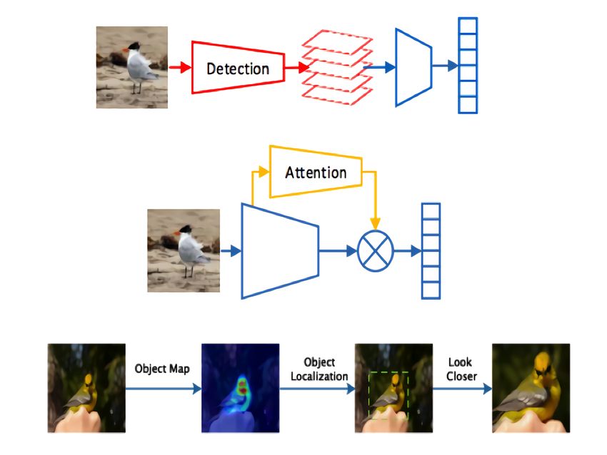
…
…
token
token
Tokens …
token
token
token
token
token
token
token
aN
LN
Attention Map LN
LN
aN-‐1
LN-‐1
LN-‐1
LN-‐1
…
…
…
a1
L1
L1
L1
a0
L0
L0
L0
Localization
Linear
Projec3on
Linear
Projec3on
Linear
Projec3on
E E E
(a) (b) (c)
Figure 2. Summary of our approach as explained in Section 2, there are three stages a,b,c, and the ViT body is shared across them. We also
show the corresponding self-attention map at stage (a) with its detected bounding box in red color.
We use a Vision Transformer (ViT) [4] for encoding im- Note that all parameters are shared across stages as in [23],
ages into feature representation for further downstream fine- and they are optimized simultaneously using the loss func-
grained classification task and use the inherent multi-head tion Ljoint defined in Equation 1, based on the Cross-
self-attention mechanism to extract attention maps with re- Entropy loss denoted as L, where La , Lb , Lc correspond
spect to the original input image using the attention flow to the three stages explained in this Section and shown in
method from Abnar et.al. [1]. Inherent multi-head self- Figure 2. Note that for stage c, Lc is the aggregation of
attention allows us to simultaneously extract features and losses from the respective N ci crops.
localize important regions in a single forward pass without
N
additional memory requirements or architectural changes. X
In our experiments we used ViT-B/16 as our encoder E and Ljoint = La + Lb + Lci (1)
i=1
a 2 layer MLP with ReLU activation in between for the
classification task. For classification, CLS token, colored The Attention Map AM is obtained by recursively multi-
in red in Figure 2, is fed to MLP. Our method composes of plying the self-attention weights a0 . . . aN from each trans-
3 stages in sequence: former layer L0 . . . LN , this recovers more information than
a Main stage: The main stage uses encoder E to extract using only the last layer.
attention maps. A bounding box is generated using the 2.1. Object Localization
object localization method. In this stage, the full image
feature is used for the downstream classification task. The attention map of the full image is binarized using a
Furthermore, the object and its corresponding attention histogram-based thresholding algorithm. Then, a grayscale
map are cropped from a higher resolution version of morphological closing is applied on this binary map. Fi-
the full image and passed down to the object stage. nally, the bounding box that covers the binary foreground
with the maximum attention value is used for object crop-
b Object stage: In the object stage, cropped image fea- ping. During our experiments, we found that mean thresh-
ture is used for the downstream classification task. olding [8] to be working well.
c Parts stage: Cropped attention map from previous
2.2. Discriminative Regions Localization
stages is used to extract fine-grained crops from the lo-
calized object image using the discriminative regions Object part regions (c) are extracted using the attention
localization method. In this stage, crops are used for map of the object after cropping it from the full attention
the downstream classification task as independent in- map as seen in (b) from Figure 2. The strength of atten-
puts. tion in local areas can be an indicator of the importance of
2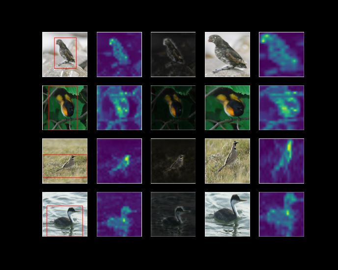
these regions captured by the model. Therefore, we search
for such regions which cover the most attention and at the
same time are not very overlapped. This allows us to find
non-overlapping object part crops. We calculate scores for
each object part region candidate in the localized object’s
attention map. These scores are calculated using Average
Pooling (AP) layer with a kernel size of H × W and stride
S = 1. Stride S = 1 is used to search all possible regions            Figure 3. Attention-based cropping and erasing (see Section 2.3).
but its value can be increased to reduce the computational
overhead. We empirically found that Max Pooling layer
leads to worse performance as it is too localized. How-
ever, generalized-mean (GeM) pooling can also be used                          Datasets           Category      Training       Testing
[18]. Kernel size of H × W is a hyper-parameter that can
                                                                          CUB-Birds [22]             200          5994         5794
be tuned based on the dataset. In our experiments, we used
                                                                        Stanford Dogs [11]           120         12000          8580
0.3 of the cropped object area, which roughly accounts for
                                                                         Stanford Cars [12]          196          8144          8041
a kernel size of 112x112 when object attention maps are re-
                                                                        Plant Pathology [17]          5          9436          12595
sized to 384 px. After the scoring, we apply Non-Maximum
Suppression (NMS) similar to other well know detectors [7]
                                                                                        Table 1. Summary of Datasets.
to get the top non-overlapping regions. We used the top 2
object regions after NMS.

2.3. Attention-based Augmentations                                             Method            Backbone         Accuracy(%)
                                                                            MaxEnt [5]        DenseNet-161              83.6
    Data augmentation allows to increase the variety of train-              FDL [REF]         DenseNet-161              84.9
ing data, prevent overfitting and improve the performance                   RA-CNN [6]          VGG-19                  87.3
of deep models. However, in FGVC, random data augmen-                       Cross-X [15]       ResNet-50                88.9
tation, such as random image cropping, is low-efficiency                    API-Net [26]       ResNet-101               90.3
and might remove informative parts. Inspired by WS-DAN                        ViT [4]           ViT-B/16                91.7
[10], we augment the image using the learned self-attention
                                                                                 Ours            ViT-B/16               93.2
map, which represents the importance of image parts (to-
kens) based on the model. As shown in Figure 3, we per-               Table 2. Comparison of different methods on Stanford Dogs and
form cropping and erasing. Removing currently attended                ablation of our method.
pixels enforces the model to consider other discriminative
regions and allows feature diversity during training. In a
given batch, we randomly apply random erasing on an im-
age with a probability P by erasing all the pixels that have                    Method              Backbone         CUB        Cars
an attention value higher than the threshold T. Particularly
RandomErasing [25], as a destructive augmentation, has                      VGG-16 [19]             VGG-16           77.8       85.7
proven to improve accuracy performance on fine-grained                     ResNet-101 [9]          ResNet-101        83.5       91.2
classification [3, 10].                                                   Inception-V3 [20]       Inception-V3       83.7       90.8
                                                                            RA-CNN [6]              VGG-19           85.3       92.5
                                                                             MaxEnt [5]          DenseNet-161        86.6       93.0
3. Experiments                                                              Cross-X [15]           ResNet-50         87.7       94.6
                                                                              DCL [2]              ResNet-50         87.8       94.5
    In this section we report the results for each benchmark                API-Net [26]         DenseNet-161        90.0       95.3
dataset. In each experiment we used the same setup for                      WS-DAN [10]           Inception v3       89.4       94.5
training. We use augmentations proposed in Section 2.3 to-                 MMAL-Net [23]           ResNet-50         89.6       95.0
gether with standard augmentations (e.g. horizontal flip, ad-                 ViT [4]               ViT-B/16         89.4       92.8
ditive noise, etc.) Full images (stage a) are resized to 384 px                  Ours               ViT-B/16         91.0       94.3
resolution in main stage, objects (stage b) and crops (stage
c) are cropped from a higher resolution and then resized to           Table 3. Comparison with state-of-the-art methods on CUB-200-
384 px before the forward pass to the next stage.                     2011 and Stanford Cars.

                                                                  3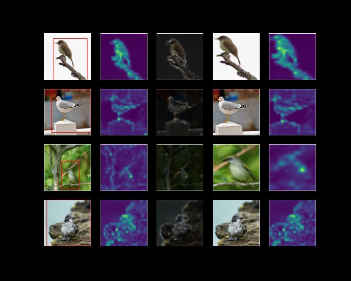
(a)         (b)          (c)        (d)          (e)         (a)         (b)        (c)          (d)         (e)

Figure 4. Results for CUB-200-2011 Dataset [22]. We show (a) input image, (b) attention map, (c) image after applying the global
attention map, highlighting informative regions, (d) attention crop, from the predicted red bounding box and (e) crop’s attention map.
These qualitative visualizations prove the effectiveness and the interpretability of our method. 8 complete results. Best viewed in color.

            Method          Backbone        Accuracy(%)
         ResNet [9]               50            89.2
       EfficienNet[21]            B0            90.1
       EfficienNet[21]            B2            90.4
           ViT [4]             ViT-B/16         91.7
             Ours              ViT-B/16         92.4

    Table 4. Method comparison on FGVC7 Plant Pathology.
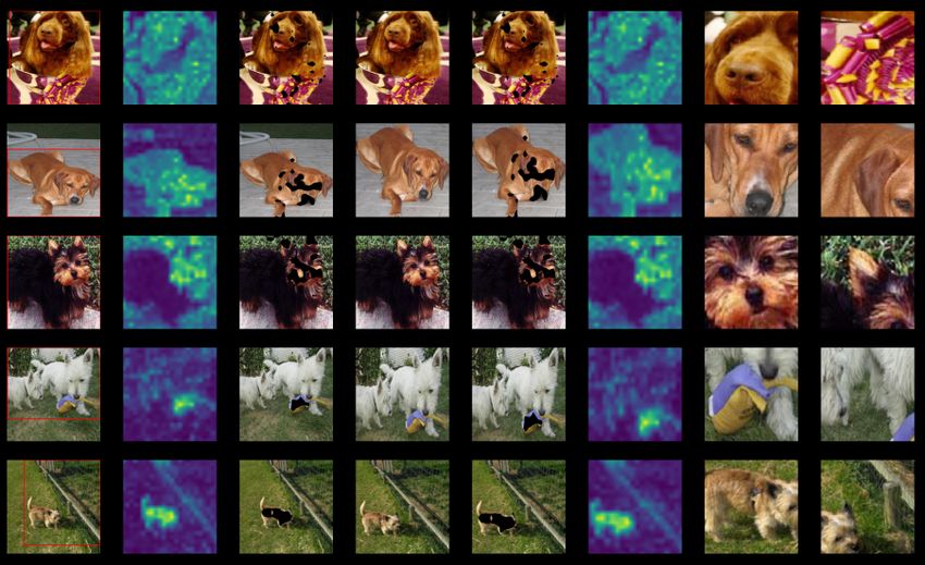
                                                                        Figure 5. Qualitative results for Stanford Dogs [11]. We show 3
                                                                        samples, from left to right: the input image with the predicted
3.1. Results                                                            bounding box (red color), the global attention map, attention-
    The reported results in Tables 2,3,4 show that Vision               based erasing augmentation (RandomErasing), selected crops and
Transformers have great potential on FGVC. Moreover, our                their attention map, the top-2 most informative regions in the im-
                                                                        age based on crop’s attention (Section 2.2). Best viewed in color.
experiments show that attention-driven augmentations and
important regions detection help to improve their perfor-
mance on fine-grained classification, achieving state-of-the-
                                                                        We aim to exploit this property in our framework, and by
art performance in Stanford Dogs [11] and CUB-200-2011
                                                                        doing it we achieve state-of-the-art results on popular fine-
[22]. However, we must expose the limitations of the pro-
                                                                        grained benchmarks. We also employ different attention-
posed multi-branch multi-scale architecture: (i) the selec-
                                                                        guided augmentations to improve our model’s generaliza-
tion of the region of interest (ROI) based on the attention
                                                                        tion capability by enforcing the model to learn more diverse
map is not fully differentiable, and thus, the model is not
                                                                        discriminative features. As future work, we aim towards
complete end-to-end trainable, it requires to train it in a se-
                                                                        making our framework end-to-end trainable and improve
quential (multi-stage) way. (ii) ViT-based models require
                                                                        this approach by exploring detection transformers.
important computational power.

4. Conclusion                                                           References
   In this paper, we propose a multi-stage multi-scale fine-             [1] Samira Abnar and Willem Zuidema. Quantifying attention
grained visual classification framework based on ViT. The                    flow in transformers, 2020. 2
multi-head self-attention mechanism can capture discrimi-                [2] Yue Chen, Yalong Bai, Wei Zhang, and Tao Mei. Destruction
native image features from multiple diverse local regions.                   and construction learning for fine-grained image recognition.

                                                                    4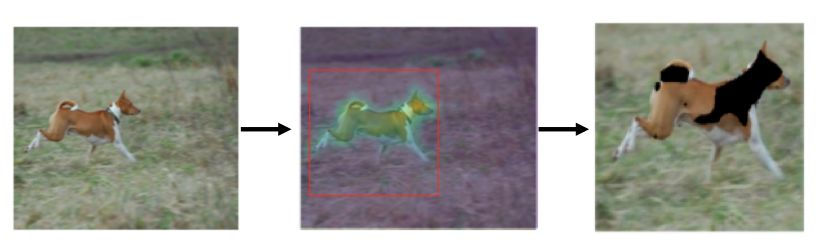
In Proceedings of the IEEE/CVF Conference on Computer               [17] Ernest Mwebaze, Timnit Gebru, Andrea Frome, Solomon
       Vision and Pattern Recognition (CVPR), June 2019. 1, 3                   Nsumba, and Jeremy Tusubira. icassava 2019 fine-grained
 [3]   Yue Chen, Yalong Bai, Wei Zhang, and Tao Mei. Destruction                visual categorization challenge, 2019. 3
       and construction learning for fine-grained image recognition.       [18] Filip Radenović, Giorgos Tolias, and Ondřej Chum. Fine-
       In Proceedings of the IEEE/CVF Conference on Computer                    tuning cnn image retrieval with no human annotation, 2018.
       Vision and Pattern Recognition (CVPR), June 2019. 1, 3                   3
 [4]   Alexey Dosovitskiy, Lucas Beyer, Alexander Kolesnikov,              [19] Karen Simonyan and Andrew Zisserman. Very deep convo-
       Dirk Weissenborn, Xiaohua Zhai, Thomas Unterthiner,                      lutional networks for large-scale image recognition, 2015. 1,
       Mostafa Dehghani, Matthias Minderer, Georg Heigold, Syl-                 3
       vain Gelly, Jakob Uszkoreit, and Neil Houlsby. An image is          [20] Christian Szegedy, Wei Liu, Yangqing Jia, Pierre Sermanet,
       worth 16x16 words: Transformers for image recognition at                 Scott Reed, Dragomir Anguelov, Dumitru Erhan, Vincent
       scale, 2020. 1, 2, 3, 4                                                  Vanhoucke, and Andrew Rabinovich. Going deeper with
 [5]   Abhimanyu Dubey, Otkrist Gupta, Ramesh Raskar, and                       convolutions, 2014. 1, 3
       Nikhil Naik. Maximum-entropy fine grained classification.           [21] Mingxing Tan and Quoc Le. EfficientNet: Rethinking model
       In S. Bengio, H. Wallach, H. Larochelle, K. Grauman, N.                  scaling for convolutional neural networks. In Kamalika
       Cesa-Bianchi, and R. Garnett, editors, Advances in Neural                Chaudhuri and Ruslan Salakhutdinov, editors, Proceedings
       Information Processing Systems, volume 31. Curran Asso-                  of the 36th International Conference on Machine Learning,
       ciates, Inc., 2018. 3                                                    volume 97 of Proceedings of Machine Learning Research,
 [6]   Jianlong Fu, Heliang Zheng, and Tao Mei. Look closer to                  pages 6105–6114. PMLR, 09–15 Jun 2019. 1, 4
       see better: Recurrent attention convolutional neural network        [22] C. Wah, S. Branson, P. Welinder, P. Perona, and S. Belongie.
       for fine-grained image recognition. In Proceedings of the                The Caltech-UCSD Birds-200-2011 Dataset. Technical Re-
       IEEE Conference on Computer Vision and Pattern Recogni-                  port CNS-TR-2011-001, California Institute of Technology,
       tion (CVPR), July 2017. 3                                                2011. 1, 3, 4
 [7]   Ross Girshick. Fast r-cnn, 2015. 3                                  [23] Fan Zhang, Meng Li, Guisheng Zhai, and Yizhao Liu. Multi-
 [8]   C.A. Glasbey. An analysis of histogram-based thresholding                branch and multi-scale attention learning for fine-grained vi-
       algorithms. CVGIP: Graphical Models and Image Process-                   sual categorization, 2020. 1, 2, 3
       ing, 55(6):532–537, 1993. 2                                         [24] H. Zheng, J. Fu, Z. Zha, and J. Luo. Looking for the devil in
 [9]   Kaiming He, Xiangyu Zhang, Shaoqing Ren, and Jian Sun.                   the details: Learning trilinear attention sampling network for
       Deep residual learning for image recognition, 2015. 1, 3, 4              fine-grained image recognition. In 2019 IEEE/CVF Confer-
[10]   Tao Hu, Honggang Qi, Qingming Huang, and Yan Lu.                         ence on Computer Vision and Pattern Recognition (CVPR),
       See better before looking closer: Weakly supervised data                 pages 5007–5016, 2019. 1
       augmentation network for fine-grained visual classification,        [25] Zhun Zhong, Liang Zheng, Guoliang Kang, Shaozi Li, and
       2019. 1, 3                                                               Yi Yang. Random erasing data augmentation, 2017. 3
[11]   Aditya Khosla, Nityananda Jayadevaprakash, Bangpeng                 [26] Peiqin Zhuang, Yali Wang, and Yu Qiao. Learning attentive
       Yao, and Li Fei-Fei. Novel dataset for fine-grained image                pairwise interaction for fine-grained classification, 2020. 3
       categorization. In First Workshop on Fine-Grained Visual
       Categorization, IEEE Conference on Computer Vision and
       Pattern Recognition, Colorado Springs, CO, June 2011. 1, 3,
       4
[12]   Jonathan Krause, Michael Stark, Jia Deng, and Li Fei-Fei.
       3d object representations for fine-grained categorization. In
       4th International IEEE Workshop on 3D Representation and
       Recognition (3dRR-13), Sydney, Australia, 2013. 3
[13]   Alex Krizhevsky, Ilya Sutskever, and Geoffrey E. Hinton.
       Imagenet classification with deep convolutional neural net-
       works. NIPS’12, page 1097–1105, Red Hook, NY, USA,
       2012. Curran Associates Inc. 1
[14]   Michael Lam, Behrooz Mahasseni, and Sinisa Todorovic.
       Fine-grained recognition as hsnet search for informative im-
       age parts. In Proceedings of the IEEE Conference on Com-
       puter Vision and Pattern Recognition (CVPR), July 2017. 1
[15]   Wei Luo, Xitong Yang, Xianjie Mo, Yuheng Lu, Larry S.
       Davis, Jun Li, Jian Yang, and Ser-Nam Lim. Cross-x learn-
       ing for fine-grained visual categorization, 2019. 3
[16]   Subhransu Maji, Esa Rahtu, Juho Kannala, Matthew
       Blaschko, and Andrea Vedaldi. Fine-grained visual classi-
       fication of aircraft, 2013. 1

                                                                       5
You can also read


