Fault diagnosis of electric submersible pump tubing string leakage
←
→
Page content transcription
If your browser does not render page correctly, please read the page content below
E3S Web of Conferences 245, 01042 (2021)                                                               https://doi.org/10.1051/e3sconf/202124501042
AEECS 2021

         Fault diagnosis of electric submersible pump tubing string
         leakage

         Jiali Yang1,†, Wei Li2,3,†, Jiarui Chen1 and Sheng Li1,*
         1 School of Mathematics and Computer, Guangdong Ocean University, Zhanjiang Guangdong,524088, China
         2 Southern Marine Science and Engineering Guangdong Laboratory (Zhanjiang), Zhanjiang, Guangdong, 524088, China
         3 CNOOC China Limited ZhanJiang Branch, Zhanjiang, Guangdong, 524057, China

         † These authors contributed equally to this work.

                       Abstract. With the rapid development of the offshore oil industry, electric submersible pumps have become
                       more and more important. They are the main pumping equipment in oil well production and have huge
                       advantages in terms of displacement and production costs. Due to the complex structure of the electric
                       submersible pump, the bad working environment will cause failures. The failure of tubing string leakage is a
                       common failure in oilfields; tubing string leakage of the electric submersible pump will reduce oil production.
                       In order to reduce the economic loss of oil well production.This paper uses PCA and Mahalanobis distance to
                       make the tubing Fault diagnosis of leakage. The feasibility of the algorithm is verified through experiments.
                       The result shows that it can diagnose the failure time of pipe string leakage in advance and hence help us to
                       reduce the maintenance cost of offshore oilfields.

                                                                              it is necessary to conduct in-depth research on the fault
                                                                              diagnosis technology of electric submersible pumps, apply
       1 Introduction                                                         new methods and new technologies to fault diagnosis of
       Electric submersible centrifugal pump (electric                        electric submersible pumps, ensure that the electric
       submersible pump) is a kind of multi-stage centrifugal                 submersible pumps work better, and create better
       pump that works in the well. It uses tubing to lower the               economic benefits for enterprises.
       centrifugal pump and the submersible motor into the well.                   At present, Peng Long et al[3]proposes a fault
       The motor drives the multi-stage centrifugal pump to                   diagnosis of the broken shaft of a submersible electric
       rotate to generate centrifugal force, which reduces the                pump based on principal component analysis, and
       crude oil in the well oil extraction equipment lifted to the           concludes that the principal component analysis algorithm
       ground. The electric submersible pump oil production                   has the potential to be used to detect dynamic changes in
       process is widely used in high water cut wells, non-self-              data. Matthews et al[4]. used random forest to classify and
       blown high-yield wells and offshore oil fields due to its              identify 7 types of oil well faults with an accuracy of 94%.
       simple equipment structure, large displacement, high                   Lu Li et al[5] used electric submersible pump wellhead
       efficiency and high degree of automation[1]. Electric                  electrical parameters and production parameters to extract
       submersible pumps can lift crude oil to the surface under              the parameter characteristics of different faults through
       conditions of higher temperature and greater depth, but                digital signal processing, and analyzed 9 types of faults.
       electric submersible pump wells are prone to failures                  Data analysis is carried out for typical fault conditions.
       during the production process, which will cause                        Zhang Panlong et al[6] proposed an algorithm based on
       production interruptions and cause serious economic                    feature extraction to diagnose electric submersible pump
       losses[2].                                                             system faults, experiments show that the algorithm can
           Under normal circumstances, once the electric                      achieve the expected goal well.
       submersible pump fails, it needs to perform workover                        This paper uses principal component analysis and
       operations, which costs a high maintenance fee, which                  Mahalanobis distance algorithm to study the daily
       brings a heavy economic burden to the oil field enterprise,            production data of electric submersible pumps. First, the
       and also affects the normal production of the oil field. It            data is preprocessed, then the principal component
       mainly relies on manual calculations and expert                        analysis algorithm is used to extract the principal
       experience to carry out post-mortem evaluation and                     components, and finally the electric submersible pump
       forecasting. There are problems such as heavy workload,                data is faulted through Mahalanobis distance. Diagnosis
       poor timeliness and low forecast accuracy, which cannot                and analysis of experimental results show that this set of
       meet the needs of modern oilfield production. Therefore,               algorithms can diagnose pipe string leakage failures in

         *Corresponding   author’s e-mail: lish_ls@gdou.edu.cn and lish_ls@sina.com

  © The Authors, published by EDP Sciences. This is an open access article distributed under the terms of the Creative Commons Attribution License 4.0
  (http://creativecommons.org/licenses/by/4.0/).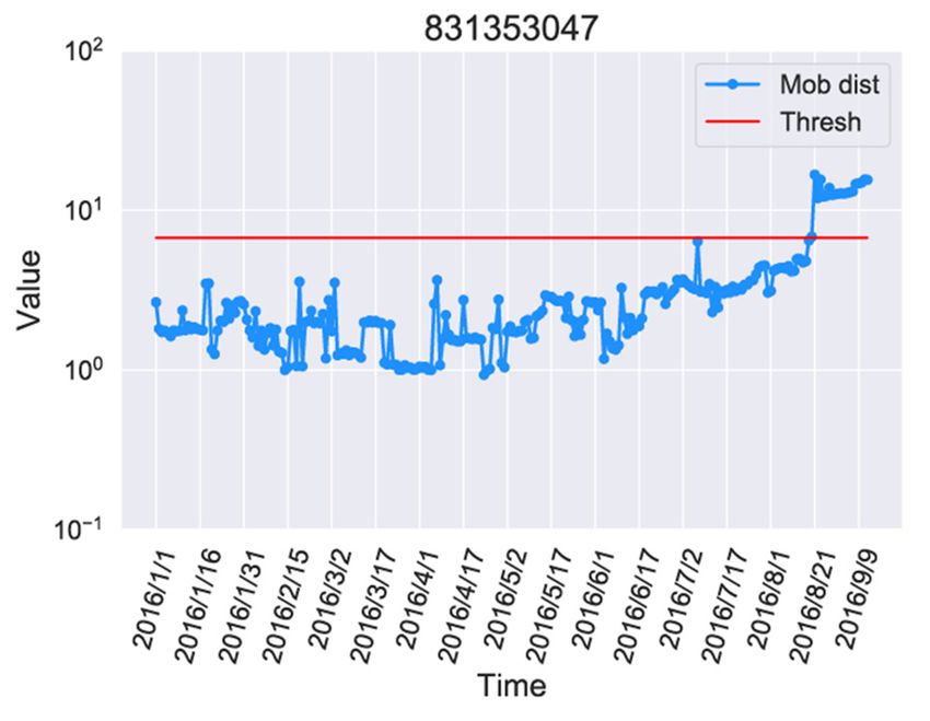
E3S Web of Conferences 245, 01042 (2021) https://doi.org/10.1051/e3sconf/202124501042
AEECS 2021
advance and achieve the benefit of reducing economic t11 t12 t1n x1
losses. t t t2n x2
Y 21 22 .
2 Principal component analysis
PCA(principal component analysis) is a multivariate tm1 tm 2 tmn xn (5)
statistical method. It is one of the most commonly used
dimensionality reduction methods. A set of potentially
correlated variable data is transformed into a set of linearly 3 Mahalanobis distance
uncorrelated variables through orthogonal transformation.
The transformed variable is called main ingredient[7]. That The Mahalanobis distance was developed by Indian
is, given a set of variables x1 , x2 ,..., xn , through a linear statistician P. C. Mahalanobis to measure the covariance
distance of data. It is an effective method to calculate the
transformation, transformed into a set of uncorrelated similarity of two unknown samples. Compared with
variables Y1 , Y2 ,..., Yn , in this transformation, the total Euclidean distance, Mahalanobis distance has more
variance of the variables (the sum of variances) is kept advantages and is not affected by dimension, that is, the
unchanged, and the maximum variance is called the first Mahalanobis distance between two points has nothing to
principal component. At the same time, Y1 has the largest do with the original data, and the calculation speed is fast.
variance, called the first principal component; Y2 has the Moreover, the Mahalanobis distance can consider the
second largest variance, called the second principal relation between various characteristics and eliminate the
component. By analogy, once there were n variables, you correlation interference between variables. To sum up,
can convert n principal components, and find out that most Mahalanobis distance can easily measure the distance
of the variance variables that can reflect the original n between the observed sample and the known sample set,
variables are p(p≤n). so it is suitable for fault diagnosis[8]. Y (Y1 , Y2 ,..., Yp ) is
First calculate the correlation between variables
the p-dimensional principal component obtained through
γij i, j 1,2,..., n , where γij γ ji . data principal component analysis, where the mean vector
is μ , the covariance matrix is Σ , and
x x
m
ki xi kj xj y ( y1 , y2 ,..., ym ) is a random sample obtained by
γij k 1
. (1) principal component analysis of Y . Then the
2 1/2
m 2 m
xki xi xkj x j
Mahalanobis distance DM from Y to the mean vector μ is:
1/2
k 1 DM Y , μ Y μ Σ 1 Y μ
k 1 T
,
Set a correlation matrix R as follows, (6)
where P is the dimension of the sample, M is the size
γ11 γ12 γ1n
of the sample.
γ γ22 γ2n
21 The μ value is calculated as followed:
R .
1 m
μ yi ,
p i 1
γm1 γm 2 γmn (2)
(7)
where the covariance matrix is:
Calculate the eigenvalue λ of the matrix, and obtain
1 m
the variance contribution rate and the cumulative variance
yi μ yi u .
'
contribution rate as the formula. p 1 i 1 (8)
λi
Fi n
, i 1, 2,..., n ,
λ
k 1
k 4 Fault Diagnosis Process
(3)
The electric submersible pump data collected by the
i
sensor has many missing and abnormal data, so the data
λ k
should be cleaned first, and then the data should be
standardized. For some attributes, only unique values need
Si k 1
n
, i 1, 2,..., n . to be deleted. Then, the preprocessed data were analyzed
λ
k 1
k
by principal component analysis to calculate variance
contribution rate and cumulative variance contribution
(4)
Finally, the principal component is: rate, and each principal component. Finally, the data set is
divided, the Markov distance and the maximum Markov
distance of the training set are calculated, and then the new
data is tested to diagnose the time of failure. The specific
fault flow is as shown in Figure 1.
2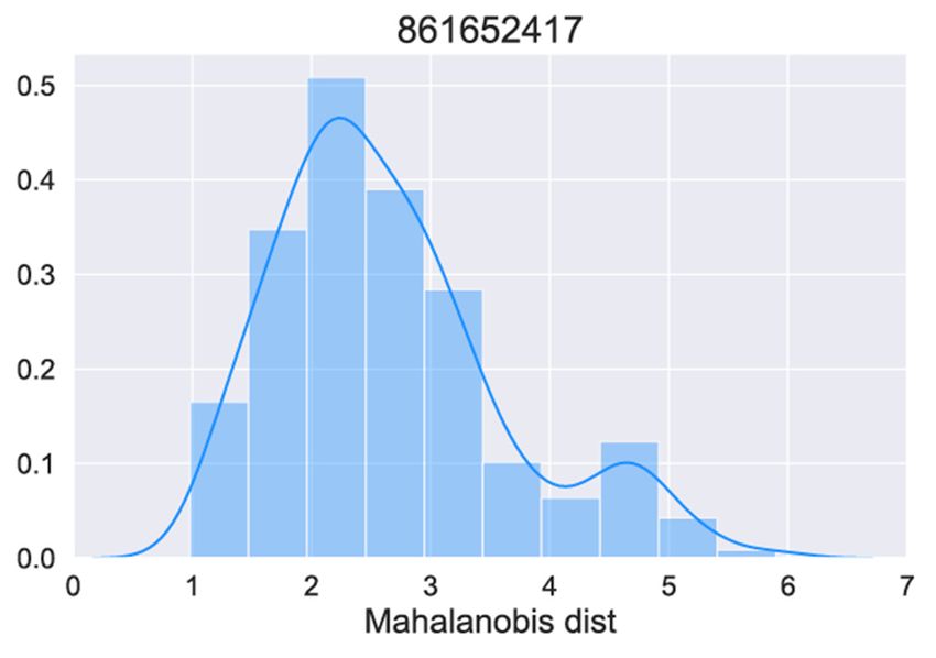
E3S Web of Conferences 245, 01042 (2021) https://doi.org/10.1051/e3sconf/202124501042
AEECS 2021
Diagnose when the fault
occurred
ESP database Data cleaning
Calculate the Mahalanobis
distance of the test sample
Data transformation
Data of ESP to be
tested
Calculate variance Calculate the Mahalanobis
contribution rate and Principal component distance and get the
Create data set maximum value of
cumulative variance analysis
contribution rate Mahalanobis distance under
the sample without failure
Draw scatters plot of
No fault ESP data
principal component
1 and 2
Figure 1. Fault diagnosis flow
5 Case study: diagnosis of the ESP
5.2. Data preprocessing
Tubing String Leakage
5.2.1. Data cleaning. Through data analysis, data
5.1. Data source of the ESP Tubing String cleaning is divided into the following steps:
Leakage
Daily measurement data of oil and gas wells are
The data in this article comes from the China National recorded multiple times a day at some time points,
Offshore Oil Development and Production Database. The and one piece of data should be retained.
sensor records the daily data of electric submersible The daily measurement data of oil and gas wells
pumps (one record per day), among which 25 oil wells is not recorded every day but is recorded
have recorded string leakage. Through data observation, irregularly (sometimes once every two or three
only the historical data of 14 oil wells can be used. The days, sometimes every five or six days), so linear
well IDs are 831352627, 831353047, 831412597, interpolation of the measurement data is required.
832012687, 833155477, 834652657, 834952567, The daily status data of oil and gas wells, the
835852627, 861652417, 861652717, 951352447, daily metering data of oil and gas wells, and the
951352747, 951412537 and 951412567. There are four daily distribution data of oil and gas wells have
different types of data sets for oil well data. They includes: been merged at the same point in time.
Daily status data of oil and gas wells: time, nozzle Delete the samples whose production time is 0,
diameter, production time, bottom hole pressure, this kind of data will lead to fault misjudgment.
wellhead temperature, oil pressure, casing Delete variables with a single value, such as
pressure, surface casing pressure, technical nozzle diameter, surface casing pressure,
casing pressure, pump current, pump voltage, technical casing pressure, etc. These variables
pump frequency, pump inlet temperature, have no effect on the data.
moisture content.
Daily measurement data of oil and gas wells:
converted daily fluid production, converted daily 5.2.2. Data transformation. Data standardization is
oil production, converted daily water production, performed on the cleaned electric submersible pump data.
converted daily gas production, test fluid volume, Because the difference between different variables is large,
test oil volume, test water volume, test gas the calculated relationship coefficients will differ greatly,
volume, wellhead temperature, oil body density, and the optimal solution of the model cannot be quickly
gas-oil ratio, water content, separator pressure, found in the optimization process. This paper uses the
separator temperature. maximum-minimum normalization method to map each
Daily distribution data of oil and gas wells: daily variable to the interval [0,1], as in equation (9).
fluid production, daily oil production, daily water
production, daily gas production, gas-oil ratio, xij xmin i 1, 2,..., n
oil-gas ratio, water cut, water-gas ratio. xij' , .
xmax xmin j 1, 2,..., m (9)
Fault information data: the data information
contains the specific time when the string leakage xmin is the minimum value of xij xmax is
occurred in each oil well. where ,
xij m
the maximum value of , is the data sample size,
3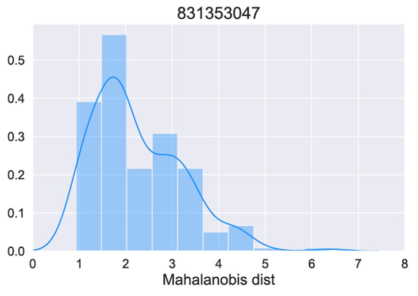
E3S Web of Conferences 245, 01042 (2021)                                                           https://doi.org/10.1051/e3sconf/202124501042
AEECS 2021

       and    n is the characteristic dimension of the data.               of data samples are distributed in the lower left corner
                                                                           (normal samples), and only a few data samples are
                                                                           distributed on the right and far from the left (faulty
       5.3. Principal component analysis                                   samples). Therefore, the two-dimensional curves of
       According to the data variables obtained by data                    principal component 1 and principal component 2 are very
       preprocessing, input the principal component analysis               important for real-time monitoring of the performance of
       model. According to the decreasing order of the variance            the electric submersible pump. If the sample starts to
       of the principal components, the different principal                deviate from the concentrated area, it can send an early
       components are sorted. Taking the well ID=831353047 as              warning of potential failure to the field engineer.
       an example, through data preprocessing, an oil well has 18
       parameters including wellhead temperature, pump current,
       pump voltage, oil pressure, daily gas production, daily
       liquid production, daily oil production, daily water
       production, gas-oil ratio, oil-gas ratio, water content,
       water-gas ratio, converted daily fluid production,
       converted daily oil production, converted daily water
       production, test fluid volume, test oil volume, test water
       volume. Through principal component analysis, the
       variance of the original input parameters with more than
       99% of the first six principal components can be observed,
       as shown in Figure 2. Among them, the first principal
       component and the second principal component have the
       highest variance, including 81% of the variance of the              Figure 3. Well 831353047 scores plot of Principal Component
       original data.                                                                      1 and Principal Component 2

                                                                           5.4. Mahalanobis distance fault diagnosis
                                                                           Extract more than 99% of the principal components of the
                                                                           original data. Well ID=831353047 as an example, extract
                                                                           the first 6 principal components to construct a data set, use
                                                                           the Mahalanobis distance model to train the data, calculate
                                                                           the Mahalanobis distance of each sample, and get
                                                                           Maximum Mahalanobis distance, and use this data value
                                                                           as the failure threshold. Through data visualization, the
                                                                           calculated threshold for marking anomalies is about 6.74,
                                                                           as shown in Figure 4.
                                                                               Through the Mahalanobis distance of the training set
                                                                           and the test set, and the calculated threshold for marking
             Figure 2. Cumulative variance contribution rate of well       anomalies. The next step is to compare the Mahalanobis
                      831353047 by principal components                    distance of the data set with the threshold. When it is
                                                                           greater than the threshold, it is marked as abnormal. As
           Figure 3 shows the distribution of the two-dimensional          shown in Figure 5, it can be seen that the oil well was
       scatter plot samples of principal component 1 and                   abnormal after 2016/8/15, but the actual failure the date
       principal component 2. It can be seen that a large number           was 2016/8/22.

                             Figure 4. Mahalanobis distance                           Figure 5. Predict date of failure

                                                                       4
E3S Web of Conferences 245, 01042 (2021) https://doi.org/10.1051/e3sconf/202124501042
AEECS 2021
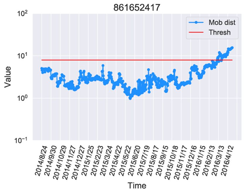
Similarly, taking the well ID=861652417 as an 2016/3/10, and the actual failure date was 2016/3/16,as
example, the threshold for marking anomalies is about shown in the Figure 6 and Figure 7.
7.96. It was detected that the oil well was abnormal on
Figure 6. Mahalanobis distance Figure 7. Predict date of failure
Table 1 shows the comparison between the calculation predicted by the Mahalanobis distance diagnostic model is
of the abnormal threshold value and the prediction of the earlier than the actual pipe string leakage time. Therefore,
string leakage of the electric submersible pump using the the Mahalanobis distance diagnosis model has excellent
Mahalanobis distance model and the actual time. The accuracy in predicting the leakage time of the electric
analysis in Table 1 shows that the pipe string leakage time submersible pump string.
Table 1. Mahalanobis distance threshold and failure prediction date and true date for each well
Well ID. MD Threshold Predict date of failure Actual date of failure
831352627 7.96 2017/3/14 2017/3/22
831353047 6.74 2016/8/15 2016/8/22
831412597 6.32 2017/7/6 2017/7/13
832012687 9.14 2019/11/18 2019/12/18
833155477 10.81 2019/7/13 2019/8/29
834652657 7.35 2019/4/26 2019/5/7
834952567 8.43 2019/4/17 2019/7/12
836452927 10.16 2019/5/9 2019/5/17
861652417 7.96 2016/3/10 2016/3/16
861652717 7.88 2018/9/12 2018/10/2
951352447 8.32 2018/12/9 2018/12/23
951352747 7.87 2015/7/28 2015/8/15
951412537 7.68 2016/5/9 2016/6/1
951412567 7.96 2018/3/13 2018/3/14
6 Conclusions Acknowledgements
This paper proposes a fault diagnosis model based on This work was supported by the Fund of Southern Marine
principal component analysis and Mahalanobis distance to Science and Engineering Guangdong Laboratory
detect the leakage fault of the electric submersible pump (Zhanjiang) (ZJW-2019-04) and the Natural Science
string in advance. Firstly, the principal component 1 and Foundation of Guangdong Province (2018A030307062).
principal component 2 can be used to judge the normal
sample and the abnormal sample, and then the
Mahalanobis distance can be used to diagnose the time References
when the fault occurs, which reduces the economic loss of 1. Xie, W., Chen, L., Wei, H.G., et al. (2017) "Multi-
oil well production. Split VVVF" System for Electric Submersible Pump
on Extraction Flat Roof on the Sea. In: Proceedings
of the 2016 6th International Conference on
5E3S Web of Conferences 245, 01042 (2021) https://doi.org/10.1051/e3sconf/202124501042
AEECS 2021
Advanced Design and Manufacturing Engineering
(ICADME 2017). Zhuhai. pp. 506-511.
2. Reges, G., Fontana, M., Ribeiro, Marcos., et al. (2020)
Electric submersible pump vibration analysis under
several operational conditions for vibration fault
differential diagnosis. J. Sci. Ocean Engineering., pp.
108249-.
3. Peng, L., Han, G.Q., Pagou, A.l., Shu, J. (2020)
Electric submersible pump broken shaft fault
diagnosis based on principal component analysis. J.
Sci. Journal of Petroleum Science and Engineering.,
191.
4. Marins, M.A., Barros, B.D., Santos, I.H.,
Barrionuevo, D.C., et al. (2020) Fault detection and
classification in oil wells and production/service lines
using random forest. J. Sci. Journal of Petroleum
Science and Engineering., 197.
5. Li, L., Hua, C.Q., Xu, X. (2018) Condition
monitoring and fault diagnosis of electric submersible
pump based on wellhead electrical parameters and
production parameters. J. Esci. Systems Science &
Control Engineering., 6(3): 253-261.
6. Zhang,P.L., Chen, T.K., Wang, G.C., Peng, C.Z.
(2017) Ocean Economy and Fault Diagnosis of
Electric Submersible Pump applied in Floating
platform. J. Esci. International Journal of e-
Navigation and Maritime Economy., 6: 37-43.
7. Konopleva, L., Il’yasov, K.A., Teo, S.J., et al. (2021)
Robust intra-individual estimation of structural
connectivity by Principal Component Analysis. J. Sci.
NeuroImage., 226.
8. Ji, H.Q. (2020) Statistics Mahalanobis distance for
incipient sensor fault detection and diagnosis. J. Sci.
Chemical Engineering Science., pp. 116233-.
6You can also read