FEASIBILITY STUDY OF THE IMPLEMENTATION OF A SPACE SUNSHADE NEAR THE FIRST LAGRANGIAN POINT - DIVA
←
→
Page content transcription
If your browser does not render page correctly, please read the page content below

DEGREE PROJECT IN MECHANICAL ENGINEERING,
SECOND CYCLE, 30 CREDITS
STOCKHOLM, SWEDEN 2020

Feasibility study of the
implementation of a space
sunshade near the first Lagrangian
point

MARÍA GARCÍA DE HERREROS MICIANO

KTH ROYAL INSTITUTE OF TECHNOLOGY
SCHOOL OF ENGINEERING SCIENCES
Feasibility study of the
implementation of a space
sunshade near the first
Lagrangian point

MARÍA GARCÍA DE HERREROS MICIANO

Master in Aerospace Engineering
Date: July 15, 2020
Supervisor: Christer Fuglesang
Examiner: Christer Fuglesang
School of Engineering Sciences
Swedish title: Möjlighetsstudie av solparasoll i rymden nära
Lagrangepunt L1
III

Abstract
The lack of strong measures to avoid the possible fatal consequences of global
warming is pushing researchers to look for other alternatives such as geoengi-
neering. Within geoengineering, this study focuses on the space based solar
radiation management methods. More precisely, the project evaluates the fea-
sibility of implementing a space sun shade near the first Lagrangian point in
the Sun-Earth system within a thirty year period time from now. The study is
structured in three main blocks: spacecraft configuration, trajectory definition
and launch. An analysis looking at the minimum cost system was carried out,
starting with the definition of the mass and size of spacecraft. Furthermore, an
optimization of the trajectory was developed in order to minimize the travel
time to the vicinity of the Lagrangian point. The shades will be formed by
swarms of 10 000 m2 solar sails that will cover an area of 6.3 × 10¹² m2 with
a total mass of around 5.7 × 10¹⁰ kg. The sails will be injected into a LEO
and will start a trajectory to the vicinity of the first Lagrangian point that will
take around 2.3 years. The total cost of the project is approximated to be 10
trillion dollars. The mission appears to be feasible from a technological point
of view, with some development needed in the attitude control subsystem. The
main challenge will be the launch of all the spacecraft. A space mission of this
dimensions has never been attempted before so it will require a big advance
from the launch vehicle industry.
IV

Sammanfattning
Bristen på åtgärder för att undvika de konsekvenser som den globala uppvär-
mingen leder till, har drivit forskare att leta efter alternativa lösningar, varav
geoengineering är en av dem. Denna studie fokuserar på rymdbaserade strål-
hanteringsmetoder, mer specifikt på hur huruvida implementationer av solpa-
rasoller nära Lagrangepunkten L1 i sol-jord-systemet är möjlig eller ej. Studi-
en är strukturerad i tre huvudsakliga block: rymdskeppskonfiguration, banade-
finition och uppskjutning. Med målet att minimera kostnaderna, definierades
rymdskeppets utforming, massa och storlek. Vidare så, optimerades vägen till
närheten av L1 med avseende på att minimera tiden. Solparasollerna kom-
mer vara placerade i svärmar med en area på 10 000 m2 vardera, totalt kom-
mer solparasollerna att täcka en yta av 6.3 × 10¹² m2 med en total massa på
5.7 × 10¹⁰ kg. Solparasollerna kommer skjutas upp till LEO och därefter star-
ta sin resa till närheten av L1, vilket kommer ta cirka 2.3 år. Totala kostanden
för projektet uppskattas till 10 billioner dollar. Efter genomförd studie visades
projektet vara genomförbart sett från en teknisk synvinkel, men vidare studi-
er behövs göras för att utveckla och fastställa styrsystemet. Huvudutmaningen
kommer att vara uppskjutningen av rymdskeppen, då det kräver stora framsteg
och utveckling inom rymdindustrin.
Contents

1   Introduction                                                                                                 1
    1.1 Current Climate Situation and Policies .                 .   .   .   .   .   .   .   .   .   .   .   .   1
    1.2 Geoengineering the Climate . . . . . .                   .   .   .   .   .   .   .   .   .   .   .   .   3
    1.3 Literature Review on Space Sun Shades                    .   .   .   .   .   .   .   .   .   .   .   .   4
    1.4 Present Work . . . . . . . . . . . . . .                 .   .   .   .   .   .   .   .   .   .   .   .   5

2   Methodology                                                                                                   7
    2.1 Initial Assumptions . . . . . . . . . . . . . .                      .   .   .   .   .   .   .   .   .    7
    2.2 Launch . . . . . . . . . . . . . . . . . . . .                       .   .   .   .   .   .   .   .   .    8
        2.2.1 Launcher Selection and Assumptions                             .   .   .   .   .   .   .   .   .    8
        2.2.2 Target orbit . . . . . . . . . . . . . .                       .   .   .   .   .   .   .   .   .    9
    2.3 Trajectory . . . . . . . . . . . . . . . . . . .                     .   .   .   .   .   .   .   .   .   11
        2.3.1 Reference Frames . . . . . . . . . . .                         .   .   .   .   .   .   .   .   .   11
        2.3.2 Solar Sail Dynamics . . . . . . . . .                          .   .   .   .   .   .   .   .   .   12
        2.3.3 New Equilibrium Point . . . . . . . .                          .   .   .   .   .   .   .   .   .   15
        2.3.4 Escape Trajectory Optimization . . .                           .   .   .   .   .   .   .   .   .   15
        2.3.5 Trajectory to Sub-L1 Optimization . .                          .   .   .   .   .   .   .   .   .   16
    2.4 Spacecraft Configuration . . . . . . . . . . .                       .   .   .   .   .   .   .   .   .   18
        2.4.1 Total Mass and Size Study . . . . . .                          .   .   .   .   .   .   .   .   .   19
        2.4.2 Mass Budget . . . . . . . . . . . . .                          .   .   .   .   .   .   .   .   .   20
        2.4.3 Control . . . . . . . . . . . . . . . .                        .   .   .   .   .   .   .   .   .   21

3   Results                                                                                                      24
    3.1 Spacecraft Configuration . .     .   .   .   .   .   .   .   .   .   .   .   .   .   .   .   .   .   .   24
         3.1.1 Total Mass and Size       .   .   .   .   .   .   .   .   .   .   .   .   .   .   .   .   .   .   24
         3.1.2 Mass Budget . . . .       .   .   .   .   .   .   .   .   .   .   .   .   .   .   .   .   .   .   28
         3.1.3 Control . . . . . . .     .   .   .   .   .   .   .   .   .   .   .   .   .   .   .   .   .   .   29
    3.2 Launch . . . . . . . . . . .     .   .   .   .   .   .   .   .   .   .   .   .   .   .   .   .   .   .   31
         3.2.1 Launcher Selection .      .   .   .   .   .   .   .   .   .   .   .   .   .   .   .   .   .   .   31

                                     V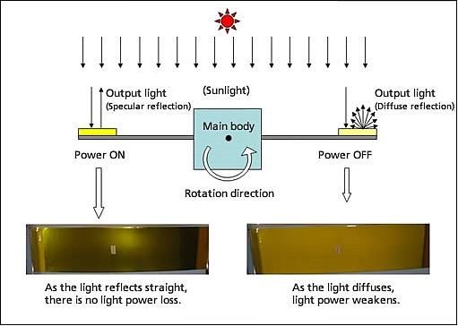
VI     CONTENTS

           3.2.2 Launch in Numbers . .        .   .   .   .   .   .   .   .   .   .   .   .   .   .   .   .   .   32
           3.2.3 Target Orbit Definition      .   .   .   .   .   .   .   .   .   .   .   .   .   .   .   .   .   33
     3.3   Final Trajectory . . . . . . . .   .   .   .   .   .   .   .   .   .   .   .   .   .   .   .   .   .   33
           3.3.1 Escape Trajectory . . .      .   .   .   .   .   .   .   .   .   .   .   .   .   .   .   .   .   34
           3.3.2 Travel to Sub-L1 . . .       .   .   .   .   .   .   .   .   .   .   .   .   .   .   .   .   .   35

4    Cost Analysis                                                         40
     4.1 Launch Cost . . . . . . . . . . . . . . . . . . . . . . . . . . . 40
     4.2 Spacecraft Cost . . . . . . . . . . . . . . . . . . . . . . . . . 41

5    Discussion                                                                                                   43
     5.1 Spacecraft . . . . . . . . . . .     .   .   .   .   .   .   .   .   .   .   .   .   .   .   .   .   .   43
     5.2 Launch . . . . . . . . . . . .       .   .   .   .   .   .   .   .   .   .   .   .   .   .   .   .   .   46
          5.2.1 Launch in Numbers . .         .   .   .   .   .   .   .   .   .   .   .   .   .   .   .   .   .   46
          5.2.2 Environmental Impact          .   .   .   .   .   .   .   .   .   .   .   .   .   .   .   .   .   47
     5.3 Trajectory Results . . . . . . .     .   .   .   .   .   .   .   .   .   .   .   .   .   .   .   .   .   49
     5.4 Cost . . . . . . . . . . . . . .     .   .   .   .   .   .   .   .   .   .   .   .   .   .   .   .   .   50

6    Conclusions                                                                                                  52
Chapter 1
Introduction
The emissions of greenhouse gases (GHG) have been changing the planet for
decades but it was not until fifteen years ago, with the Kyoto Protocol, that
climate change started to get attention from governments. Since then, the im-
portance of it has been growing. However, up to now actions against it have
not been taken with the urgency that the problem requires in order to avoid
possible fatal consequences [1] [2]. This is pushing researchers to look for
alternatives away from the reduction of greenhouse gases emissions, which as
time passes seems harder to achieve on time and requires the commitment of
the whole world [3] [4].
1.1 Current Climate Situation and Policies
Since the pre-industrial age, the world’s climate has changed significantly be-
cause of the emission of GHG, but there has been a great acceleration of these
changes in the past fifty years. The main contribution to the emissions is fossil
carbon dioxide (CO2 ), which mainly comes form energy and industrial use.
This explains the acceleration during the industrial era and specially in the last
decades.
After 2010, GHG emissions have been growing at a rate of 1.5 per cent
per year and the peak of these emissions does not seem like it is going to take
place any time soon [2]. Every year that this peak is delayed translates into a
larger rise of the global mean temperature by the end of the century. Different
scenarios are considered by the United Nations–sponsored Intergovernmental
Panel on Climate Change concluding that in order to stabilize the mean global
temperature around 2◦ C above pre-industrial levels by 2100, this peak should
12 CHAPTER 1. INTRODUCTION
take place between 2020 and 2050 [5].
By 2017 temperature had already risen 1◦ C [5] and as a consequence global
warming effects are already observable on the planet, although these will be
more intense in the following decades [6]. Some of the most important are the
rise of sea level as a result of the melting ice, the increase of extreme weather
events such as droughts, heavy rainfalls or heatwaves, the extinction of plant
and animal species, the reduction of crop fields and the increase of wildfires
[7]. All these phenomena translate in large costs for society (increase in mor-
tality, consequences in human health) and economy (damage of infrastructure,
agriculture, tourism and energy sectors).
The most recent international agreement regarding climate change was the
Paris Agreement (2016), ratified by 187 countries as of 2019. Here, all signa-
tories compromised to: “holding the increase in the global average tempera-
ture to well below 2◦ C above pre-industrial levels and pursuing efforts to limit
the temperature increase to 1.5◦ C" [8]. Therefore, the upper limit that should
not be trespassed is nowadays set to 2◦ C. It must be kept in mind that the 0.5◦ C
difference between both limits means a significant increase in the intensity of
the global warming effects mentioned above [5].
With the current climate policies and the ones expected to be implemented
in the following years, by the end of the century temperature is predicted to
rise between 2.6◦ C and 3.7◦ C, depending on the compliance with these poli-
cies [1]. Thus, it seems clear that stronger measures need to be taken to reduce
GHG emissions in order to achieve the defined goals. To meet the 1.5◦ C limit,
global CO2 emissions would need to reach zero by 2050 and keep decreasing
afterwards. This means that emissions would need to start dropping immedi-
ately at a faster rate than ever and once zero emissions were reached, carbon
removal techniques would have to be implemented [9]. The chances of achiev-
ing these objectives seem remote, specially keeping in mind that, in order to do
so, an international response needs to be coordinated on a global level. Oth-
erwise, despite all the climate policies that are being implemented in a lot of
countries, the decrease of emissions in these will not be enough to offset the
increase in others [2].CHAPTER 1. INTRODUCTION 3
1.2 Geoengineering the Climate
As it has been described before, historically the dominant approach to fight
climate change has been the reduction of GHG emissions. While the achieve-
ment of the necessary levels of emissions in time is each year further away from
reaching the goal, other alternatives are being considered in addition to these
reductions. One of the options is so-called geoengineering, which consists
on deliberately modifying Earth’s environment in order to counteract climate
change. As addressed in Geoengineering the climate. Science, governance
and uncertainty [3], these measures are still highly controversial but they are
alternatives that can provide help, mitigating both short-term and long-term
global warming effects. Despite being an important alternative to be consid-
ered, it must be acknowledged that geoengineering methods should not be seen
as a solution but as part of a larger set of measures to fight climate change.
Geoengineering techniques can be divided in two different groups: Carbon
Dioxide Removal (CDR) and Solar Radiation Management (SRM). The first
group aims to reduce the level of carbon dioxide in the atmosphere, while SRM
techniques reduce the net incoming solar radiation received at the surface of
the planet by deflecting it before reaching Earth or increasing the reflectivity
of the planet surface or its atmosphere. Inside the second group, it is possible
to find different techniques, such as the release of stratospheric aerosols, sur-
face albedo enhancement or space based techniques. Although space based
proposals are not seen as affordable given their large cost and necessary tech-
nology development, they have two important advantages compared to Earth
based techniques: they do not require the modification of the Earth surface or
atmosphere and they have a more uniform effect [3]. Furthermore, they would
be the most cost effective if long term geoengineering is necessary [3].
The implementation of the space based proposals aims to reduce the solar
radiation reaching Earth. Theoretical calculations [10] point out that, in order
to be able to offset the effects caused by a doubling of the carbon dioxide con-
tent in the atmosphere (compared to pre-industrial levels) the solar radiation
would need to be reduced 1.7% . This would be equivalent to reducing the
average global temperature by approximately 2◦ C [11].4 CHAPTER 1. INTRODUCTION
Table 1.1: Literature review.
Authors Year Concept Total mass (tonnes)
Mautner [12] 1991 Solar screen orbiting the Earth 108 − 109
Reflecting discs in L1 2.6 × 10⁸
McInnes [17] 2002
Absorbing discs in L1 5.2 × 10⁷
Particle rings orbiting the Earth 5 × 10⁹
Pearson et al. [13] 2002
Spacecraft rings orbiting the Earth 2.3 × 10¹²
Angel [15] 2006 Cloud of spacecraft near L1 2.3 × 10¹²
Struck [14] 2007 Dust clouds at stable lunar Lagrange points 2.1 × 10¹¹
Sánchez & McInnes [16] 2015 Discs in orbit near L1 1.4 × 10⁷
1.3 Literature Review on Space Sun Shades
Among SRM geoengineering methods, space based techniques aim to avoid
part of the solar radiation from reaching Earth’s atmosphere. The implemen-
tation of these techniques has been discussed numerous times in the literature,
considering a wide range of alternatives that can be found in Table 1.1. The
creation of reflective rings in orbits around Earth has been mentioned by dif-
ferent authors as Mautner [12] and Pearson et al. [13], but these techniques
would create a large orbital debris hazard and they could affect how light is
perceived from the surface of the planet [11]. Other options considered are
related to the use of stable points in space to place these reflectors, both in
the Moon-Earth system (Struck [14]) and the Sun-Earth system (Angel [15],
Sánchez and McInnes [16], McInnes [17]). Out of these, the most effective
method so far appears to be the use of the L1 point in the Earth-Sun system
[11], since the use of the Earth-Moon system stable points would only allow
to reduce solar radiation for a certain period of time each month. On the con-
trary, the use of the first Lagrange point, which is located in the Sun-Earth line,
would reduce solar radiation the whole time the reflector is in place.
The type of reflectors used to avoid sunlight from reaching Earth has also
been discussed as well as where they should be manufactured. Struck [14],
Pearson et al. [13] and Mautner [12] considered the use of clouds of dust par-
ticles that should be obtained from asteroids or the moon surface. Other and
more recent authors consider different kinds of spacecraft, with various levels
of control over their movement. Angel [15] proposes the use of a large number
of small and light vehicles placed in a random cloud with little control, mean-
while Sánchez and McInnes [16] present two discs in a certain controlled orbit
close to the L1 point. As pointed out by McInnes [17], the large discs proposed
would need to be manufactured in space, while a smaller spacecrafts could beCHAPTER 1. INTRODUCTION 5
manufactured on Earth, as Angel [15] describes.
Comparing the mass to make these studies a reality, as it can be seen in
Table 1.1, the lightest option proposed is the most recent one [16], but the
mass of the system is not always a driver in this case. For those proposals built
in space, the mass is not a constraining factor. Although a new constraining
factor appears here, which is the necessary advance in technology to be able
to mass produce in space, which so far is not even contemplated.
1.4 Present Work
The aim of this project is to study the feasibility of the realization of space
based geoengineering ideas in the near future. Considering the studies de-
scribed in section 1.3, among all these methods, the alternative which is ap-
parently more effective is the deployment of large discs in the vicinity of the
first Lagrange point.
One of the problems faced by the most common space based techniques
proposed is that, even though a uniform reduction of the solar radiation would
decrease the global mean temperature, the effects at a regional level would
change depending on the latitude [3]. More precisely, as studied in [16], there
would be a cooling of latitudes close to the equator and a warming of the poles.
This is the reason why the most recent study regarding this type of geoengi-
neering option [16] studies the optimal configuration of the shades in order to
minimize the differences. The final result of the paper written by Sánchez and
McInnes [16] leads to the deployment of two discs orbiting around the sub-L1
point (new point resulting of the equilibrium of gravitational forces and solar
radiation pressure). From now on, it will be assumed that this is the config-
uration of the shades to be deployed. The area and exact orbit of the discs
are to be defined further in the project once the features of the spacecraft are
described.
Since the goal is to find the best mean to accomplish the deployment of
the shades in the following decades, the approach is focused on their trajec-
tory to the vicinity of the first Lagrange point, the features of the spacecraft
used regarding control and layout, and the launch of these spacecraft into or-
bit. The technologies contemplated in the project already exist or are being
developed inside the space sector, with technology readiness levels between
four and nine. As any other space mission, and specially given the dimensions6 CHAPTER 1. INTRODUCTION
of this project that can be anticipated going back to the literature study, the
leading driver during the study is the cost of the mission, which in space usu-
ally translates into mass. On a second level it is also considered the time of
the mission. The reason for the lesser importance given to the time is that the
period in which the shades should be put into place is not specifically defined.
The final goal of the shade is to avoid surpassing the 2◦ C global mean
temperature rise in order to avoid severe consequences [6]. Therefore, the
time limit for the project must be defined based on this goal. In the worst case
scenario studied in [1], which corresponds with a world where emissions keep
rising till 2100, the 2◦ C limit would be surpassed by 2050. Looking at these
results, it was decided to set this as the time limit when the shades should be
in position and operating by this year.
The first step in the study of the trajectories is the definition of the propul-
sion system used in the spacecraft to travel to the Lagrange point. It is assumed
that in the near future the production of large structures in space would not be
possible, therefore the discs would be manufactured on Earth. As a conse-
quence, the spacecraft size needs to be modified so it can be launched from
the Earth’s surface into space. Later on, once the discs are in place, the control
strategy that they will follow will be described. Next, the general layout of the
spacecraft will be addressed, focusing on the materials, the mass budget, the
size and the control techniques used, as well as the control strategy. To close
the thesis, a discussion and a conclusion will be carried out. Here the results
of the project will be commented, as well as its possible chances to become a
reality and its social effects.Chapter 2
Methodology
The feasibility evaluation of the deployment of a space sun shade in the vicinity
of the first Lagrangian point requires the analysis of certain areas, common in
any space mission. In the methodology chapter, the different approaches used
during the process are presented.
2.1 Initial Assumptions
In order to enable the selection of the trajectory for the mission there were
some aspects that needed to be clarified. As already mentioned, assuming that
in a near future the human race will not have access to the manufacturing of
large structures in space, it will not be feasible to launch the two large discs
described in [16] from Earth. For this reason, instead of using just discs, it was
decided that each one of the two shades would be composed by a certain num-
ber of smaller spacecraft, which can be put into orbit with an existing launch
vehicle (or one under development). As an initial approximation, considering
the total area described in [16] and that one spacecraft could have an area of
400 m2 , the number of spacecraft orbiting the vicinity of the L1 point would
be around 16 250 million.
Related to the travel to the sub-L1 point, the best propulsion system had to
be chosen. Two options were considered at the very beginning of the research:
electric propulsion and solar sailing. No other systems were taken into account
because they would require to carry large amounts of propellant and thus they
would greatly increase the cost of the mission. Electric propulsion is a type of
low thrust space propulsion that uses electrical power to accelerate a propel-
lant and create thrust. It has a really high specific impulse which, compared to
78 CHAPTER 2. METHODOLOGY
chemical propulsion, allows to create a low continuous thrust for long periods
of time and with small amounts of propellant. Solar sails allow spacecraft to
use solar pressure to propel themselves through space, without the need of any
kind of propellant. The attitude of the sail surface controls the thrust vector,
allowing the vehicle to travel in different directions.
The final goal of the spacecraft once in place is to cover a large area with
the lowest weight possible, which gives as a result a vehicle with a design
similar to a solar sail [16], even if this sail has never being considered to travel
through space in previous studies. Considering this and the fact that solar
sailing does not require any kind of propellant (which leads to a reduction in
the launch mass compared to any other propulsion system), it was decided that
the propulsion system best suited for the mission was solar sailing.
2.2 Launch
As outlined previously, it was assumed that the spacecraft will be launched
from Earth. Consequently, it is necessary to study the best options to put such
a large mass in orbit, regarding the type of vehicle and the orbit that this vehicle
needs to reach. In addition, the launch site selection must also be examined.
2.2.1 Launcher Selection and Assumptions
The selection of the launch vehicle is crucial to define the final cost of the mis-
sion, representing between fifteen and twenty-five percent of the total budget
in the development of a regular space mission [18]. Moreover, in this project
the launch percentage is expected to be even higher because of the large mass
of the system. Therefore the driver choosing the launch vehicle for the shade
was the price per kilogram.
The approximate mass expected for the system, using as reference the most
optimistic of the studies treated previously, is around 1.4 × 10⁷ tonnes [16].
Considering that historically the launcher with the largest payload capacity
has been the Saturn V, which stopped working in 1973 and had a capacity of
140 tonnes, the number of launches necessary to put the shade in space will
be around 105 . Since the second driver during the project was time, it was
considered that the reduction of the number of launches needed would mean
a reduction of the time it takes to put them in orbit. This together with the
fact that the price must be as low as possible, points towards the search of theCHAPTER 2. METHODOLOGY 9
Table 2.1: Launcher considered during the study.
Launcher Payload to LEO (kg) Cost ($/kg) Situation
Starship [19] 100 000 + 201 Under development
Long March 9 [20] 140 000 - Under development
SLS Block 2 [21] 130 000 8 0002 Under development
SLS Block 1B [21] 105 000 8 0003 Under development
Yenisei [22] 88 000 - 115 000 - Under development
Falcon Heavy [23] 63 000 1 430 Operational
1
Cost for SpaceX, no information about the costumer cost yet. [24]
2
Cost estimated in 2019. [21]
3
Cost estimated in 2019. [21]
cheapest launch vehicle on the market and the one with the most payload ca-
pacity, to reduce both price and number of launches needed.
The heaviest rocket currently operational is the Falcon Heavy from the
company SpaceX [23], which is able to carry around 64 tonnes to Low Earth
Orbit (LEO), but there are several launchers under development with larger
payload capacities expected to be operational in the next decade. Regarding
the cost, as it can be seen in the Table 2.1, the cheapest is the Starship devel-
oped by SpaceX, although it must be pointed out that official costs have not
been released about this launcher. The main reason for its lower price, when
compared with the rest of heavy vehicles selected in Table 2.1, is its complete
reusability.
2.2.2 Target orbit
Before starting the trip to the vicinity of the Lagrangian point the spacecraft
must escape Earth’s gravitational sphere of influence. To do so, there are two
different options to consider: the launcher injects the spacecraft directly in an
escape trajectory or the spacecraft is injected in a parking orbit, from where it
will escape the gravitational field using its own propulsion system.
The payload capacities in Table 2.1 are referred to LEO. If the spacecraft
is to be injected in an escape trajectory, the capacity for these launchers is
considerably reduced. Thus, the number of launches needed would increase
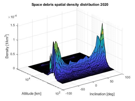
as well as the cost per kilogram of each one of these launches. Consequently10 CHAPTER 2. METHODOLOGY Figure 2.1: Space debris distribution with altitude and inclination in 2020. Data obtained from ESA MASTER 2009. it was decided that the best option was to use a parking orbit from where the spacecraft would travel by its own means of propulsion. The next step was to select the best parking orbit. The main propulsion system of the spacecraft is a solar sail. Solar sails have a large area, which means that for low Earth orbits the atmospheric drag generated by them can not be neglected. For altitudes higher than 1000 km the acceleration generated by the solar pressure on the sail is higher than the one generated by the drag [25]. If this was not the case, the solar sail will never be able to escape, therefore, altitudes below 1000 km were dismissed. Moreover, it must be taken into account that solar sails are large areas made of extremely thin materials, which makes them especially sensible to any kind of space debris. In figure 2.1 is shown how the space debris is distributed in different orbits. Based on this, it was decided that to minimize the possibilities of collision, the spacecraft should be injected at an altitude higher than 2000 km . From here, the solar sail would be deployed and the escape trajectory would start. It must be mentioned that although the space debris in altitudes higher than 2000 km is much fewer than in lower altitudes, the solar sail may face some problems when crossing the geostationary orbits zone.
CHAPTER 2. METHODOLOGY                  11

    The selection of the inclination of the parking orbit was driven by: the
possibility of cost reduction by using the Earth’s rotation boost and the launch
window available. The reduction can be achieved by taking advantage of the
Earth’s rotation when launching, which gives a boost to the vehicle and allows
to carry more payload than without it. This boost increases if the vehicle is
launched from a space port located close to the equator and to take the most
advantage out of it, the launch azimuth must be close to 90◦ . Taking into
account these two characteristics the most convenient inclination for the orbit,
regarding the cost reduction, must be close to zero. The reason for it can be
deduced from Equation 2.1 which relates the latitude (Φ), launch azimuth (β)
and inclination (i).
                               cos i = cosΦ cos β                           (2.1)
Given that the number of launches required to take the shade to space has been
calculated to be around 105 , it will be necessary to carry out several launches
a day and therefore multiple space sports around the globe must be operating.
To make sure that in all of them the launch window is as wide as possible, the
best is to place the spacecraft in an equatorial orbit. This type of orbits has a
constant launch window when launching from equatorial locations.

2.3      Trajectory
This section describes the study of the trajectory of the spacecraft once it is
released in the correct target orbit. It was decided to divide it into two phases,
since the dynamics of the vehicle are different in each one of them. First the
spacecraft will carry out an escape trajectory to exit Earth’s sphere of influence
by just using the solar sail. Once outside of the planet gravitational field, the
sail will start its way to the equilibrium point close to Sun-Earth L1 point. Both
phases were optimized in order to reduce the travel time, since the propellant
is not a driver in the case of solar sails.

2.3.1     Reference Frames
For each one of the phases different reference frames are used to study the
dynamics of the vehicle, being a total of three different reference frames:

   • Earth Centered Inertial (ECI)

   • Circular Restricted 3 Body Problem (CR3BP)
12 CHAPTER 2. METHODOLOGY
• Earth Centered Sun Pointing (ECSP)
The ECI reference frame is an inertial frame centered on the Earth that
does not rotate with respect to the stars. The x-axis points towards the vernal
equinox, the z-axis coincides with the Earth’s rotational axis and the y-axis
completes the right-handed orthogonal frame with the first two axes such as
ŷ = ẑ × x̂.
The CR3BP center is placed in the center of mass of the three body system,
which in this case is placed on the Earth-Sun line. The x-axis points towards
the Earth, the z-axis is perpendicular to the ecliptic plane and the y-axis com-
pletes the right-handed orthogonal set just as before.
Finally, the ECSP is an Earth centered system that moves with Earth rota-
tion around the Sun. Its x-axis points towards the Sun, the z-axis is perpendic-
ular to the ecliptic plane and the y-axis completes the right-handed orthogonal
set.
2.3.2 Solar Sail Dynamics
This project assumes ideal solar sails, which means that the force generated by
the solar pressure on the sail is perpendicular to its surface ( n̂ being the vector
in this direction). The acceleration that the solar radiation pressure induces in
the sail is described as: [26]
µsun
~as = β (r̂s · n̂)2 n̂ (2.2)
rs2
where µsun = 1.327 × 10²⁰ m3 s−2 is the gravitational constant of the Sun, rˆs
is the unit Sun-sail vector, rs is the Sun-sail distance and n̂ is the normal to
the sail surface in the direction of the force. The parameter β is the solar sail
lightness parameter, which is the ratio between the maximum acceleration of
the vehicle due to the Solar Radiation Pressure (SRP) and the gravity of the
Sun. This value is a function of the spacecraft areal density σ (in g m−2 ) and
the optical properties of the sail Q. Being Q = 1 a perfectly reflecting surface
and Q = 0 a surface that does not change the direction of the photons at all
[16].
1.53 · Q
β= (2.3)
σCHAPTER 2. METHODOLOGY 13
The value 1.53 represents the critical loading parameter in g m−2 . It is the
mass to area ratio that a sail, oriented perpendicular to the sun line, should
have to generate a force equal and opposite to the solar gravitational force.
The thrust vector (n̂) can be defined using two angles that describe the
orientation of the solar sail with respect the CR3BP axes: the cone angle α
that corresponds to the angle between the normal to the surface and the x-axis
and the clock angle δ which defines the angle between the normal vector and
the y-z plane. In terms of these angles, the normal vector is described with the
following expression.
n̂ = cos α, sin α cos δ, sin α sin δ (2.4)
Two-Body Problem Equations
The two body problem was solved when studying the escape trajectory of the
solar sail, while the gravitational force of Earth was the primary force acting on
it. The equations of motion of the spacecraft are written in the ECI reference
frame.
µ
~r¨ = − 3 · ~r + ~as (2.5)
|~r|
where r represents the position of the spacecraft and ~r¨ its acceleration.
Three-Body Problem Equations
Once the solar sail is outside the sphere of influence of Earth the trajectory be-
comes a three-body problem, where the gravity of the Sun also must be taken
into account. To solve this new problem, first the state vector of the sail in the
last position of the two body solution was transformed from the ECI coordi-
nates to the CR3BP reference frame. Starting at this point, the equations of
motion for the three-body problem (expressed in the CR3BP reference frame)
were used to solve the movement of the spacecraft.
Given the large dimensions of the variables that these equations were go-
ing to work with, it was decided to use dimensionless variables. In order to
do so, new units were introduced. The unit length chosen was the distance
between the Sun and the Earth (1AU); the unit of mass was defined as the sum
of the mass of these two bodies such as msun + mearth = 1; the mass ratio
µ = mearth /(msun +mearth ) and finally, the time unit selected was 1/ω, where14 CHAPTER 2. METHODOLOGY
Figure 2.2: Circular Restricted Three Body Problem schema [27]
.
ω is the angular velocity of the Earth around the Sun.
In this reference frame and with the units mentioned, the motion of the
solar sail can be described as:
~r¨ + 2ω × ~r˙ = ~as − ∇U (2.6)
where U is representing the effective gravitational potential, which can be writ-
ten as:
x2 + y 2 1−µ µ
U =− −( + ) (2.7)
2 |~r1 | |~r2 |
~r1 and ~r2, that can be seen in Figure2.2, are defined
where the position vectors
as ~r1 = x + µ y z and ~r2 = x − (1 − µ) y z . It must be stressed
that this potential represents not only the gravitational potential but also the
centripetal acceleration, included in the equation with the first term. To use
the solar sail acceleration with these new dimensionless units it needs to be
rewritten as:
1−µ
~as = β (r̂1 · n̂)2 n̂ (2.8)
(~r1 )2
where rˆ1 and n̂ are unit vectors.CHAPTER 2. METHODOLOGY 15
2.3.3 New Equilibrium Point
The first Lagrangian point is a location in space, laying on the Sun-Earth line,
where the gravitational forces of the two bodies and the centrifugal force of
the orbital motion of the third body create a stable location. Thus, a smaller
mass placed in this point remains in the same relative position. When working
with solar sails a new force needs to be taken into account, the solar radiation
pressure. As a result, the point where a third mass is in equilibrium changes
sunwards from the classical location, which is located around 1.5 × 10⁶ km
away from Earth (1/100 of the total distance between the two bodies).
To figure the new position the new force equilibrium needs to be com-
puted so the total acceleration is equal to zero. At this point the sail
will be
perpendicular to the sunlight, the normal to the surface will be n̂ = 1 0 0 .
Considering this and the fact that the point will be on the x-axis, the equation
to find the location of the new equilibrium point (xe ) is Equation 2.9 [16].
γ 5 −(3−µ)γ 4 +(3−2µ)γ 3 +(1−2µ−(β +1)(1−µ))γ 2 +2µγ −µ = 0 (2.9)
with γ = xe − (1 − µ). As it can be seen from the equation, it is possible
to change the position of the equilibrium point by selecting a certain lightness
parameter for the sail. This variation will be used later on to study the area
and total mass variation depending on the sail features.
2.3.4 Escape Trajectory Optimization
Solar sailing provides the spacecraft with very low acceleration, which leads
to that an orbital maneuver takes a long period of time. Therefore, the goal of
the escape trajectory optimization is to minimize its time.
The energy per unit mass of a body orbiting around a planet is defined as:
1
E = ~v T ~v + U (~r) (2.10)
2
where U (t) is the potential energy per unit mass and it has a negative value.
The energy of the body remains constant and negative as long as it stays in
orbit. To enable the body to escape the gravitational field, the energy must be
above zero, which can be achieved by increasing its speed.16 CHAPTER 2. METHODOLOGY
The strategy followed to achieve the escape consists in maximizing the in-
stantaneous rate of increase of orbital energy. This approach does not lead
necessarily to the minimum time solution, but it has been shown that for the
order of magnitude of solar sail acceleration the solution obtained is near min-
imum time [28]. The instantaneous rate of increase of the orbital energy is
defined in Equation 2.11 [28].
dE
= ~v˙ T ~v − g~c T ~v = a~s T ~v (2.11)
dt
It can be deduced that in order to maximize it, the component of the sail ac-
celeration along the velocity vector must be maximized in each point of the
trajectory. The optimization problem was solved by Coverstone and Prussing
[28] in the ECSP reference frame resulting in the following control law for the
normal of the sail:
− |vy |
nx = q (2.12)
vy2 + ξ 2 (vy2 + vz2 )
ny = ξnx (2.13)
vz
nz = ny (2.14)
vy
where the variable ξ is described as:
q
−3vx vy − vy 9vx2 + 8(vy2 + vz2 )
ξ= (2.15)
4(vy2 + vz2 )
Based on this result, to compute the escape trajectory of the sail the equa-
tions of motion 2.5 defined in section 2.3.2 were solved. In order to do so,
everything was transformed to ECI coordinates. The simulation was stopped
once the total energy of the sail reached zero, starting at this exact point the
second phase of the trajectory outside the sphere of influence of Earth.
2.3.5 Trajectory to Sub-L1 Optimization
The minimum-time solar sail trajectory is an optimal control problem, which
can be solved by two different methods: the indirect and the direct. For this
project the direct approach was selected, as suggested in [29]. The direct meth-
ods transform the optimal control problem in a parameter optimization prob-
lem. In order to do so, the control variables are discretized by dividing theCHAPTER 2. METHODOLOGY 17
trajectory in a certain number of segments. In the paper mentioned [29], it
was demonstrated that with few segments a near minimum-time solution can
be accomplished. During the study it was assumed that the changes between
different angles were instantaneous, which must be taken into account when
reading the final results.
Problem Definition
Any trajectory optimization problem can be described as a system of state
variables (x(t)) and control variables (u(t)). The optimal control problem is
generally defined as:
Z tf
J(x, u) = f (t, x(t), u(t))dt (2.16)
t0
ẋ = f (t, x(t), u(t)), t ∈ [t0 , tf ] (2.17)
r(x(t0 ), x(tf )) = 0 or ≥ 0 (2.18)
g(t, u(t)) ≥ 0, t ∈ [t0 , tf ] (2.19)
where J is the objective or cost function, ẋ are the state equations, r represents
the boundary conditions (initial and final) and g stands for the path constraints
defined during the trajectory. The function f represents any function depen-
dant of those variables. Next each one of the functions selected to define the
problem under study are presented.
• State and control variables. The state variables in this case are the po-
sition and velocity coordinates of the spacecraft. The control variables
are the two angles that define the normal of the solar sail, the clock angle
and cone angle, which are defined in subsection 2.3.2.
• Cost function. The cost function is the function to be optimized, which
here corresponds with the final time of the trajectory.
J = tf (2.20)
• State equations. These are equations that define the system dynamics,
therefore the equations of motion 2.6 defined in section 2.3.2.18 CHAPTER 2. METHODOLOGY
• Boundary conditions are usually defined as initial and final points of the
trajectory. The initial point is defined by the final point of the escape
trajectory, while the final point is the new equilibrium point in the Sun-
Earth line. In order to facilitate the optimization process, the final point
values were allowed to have a relative error of 10−5 .
• Path constraints are restrictions imposed to the variables that must be
respected throughout the complete trajectory, both nonlinear constraints
and upper or lower bounds.
Regarding the upper and lower bounds, none were defined for the state
and control variables. The only bounds determined for the optimization
were defined for the final time (objective function), setting the lower
bound to zero and testing the upper bound in order to get a solution.
One nonlinear constraint was set, in order to make sure that the reflective
side of the sail is pointing towards the sun all the time.
r̂ · n̂ ≥ 0 (2.21)
Multiple Shooting Parametrization Method
As it was mentioned before, the optimal control problem was solved using
a direct method that allows to treat the optimal control problem as an opti-
mization problem by discretizing the control variables. A certain number of
segments is defined to divide the trajectory, which was chosen to be ten. For
each one of these segments, the cone and clock angles have a constant value.
These parameters are the optimization variables that the optimizer will change
in the search of a solution. Thus, there are 10 × 2 optimization variables, two
per segment. The optimization was developed using the SNOPT optimization
software, which uses a sequential quadratic programming (SQP) algorithm.
The software was used on MATLAB, using the interface developed by Gill
and Wong [30].
2.4 Spacecraft Configuration
Initially, the scope of this project did not cover the definition of the spacecraft
features but, after observing how the results of its dynamics depend on it, it
was decided to developed a rough description of the layout of the spacecraft.
The areas in which the description is more precise are the ones related directly
with the performance of the solar sail, such as the sail area, the total mass of
the spacecraft and the sail material.CHAPTER 2. METHODOLOGY 19
2.4.1 Total Mass and Size Study
The main driver during the whole project was the cost and therefore the to-
tal mass. This value depends on the total area (A) needed for the shade and
the areal density of each one of the spacecraft (σ) that create this shade. This
density can change during the mission because some of the elements can be
jettisoned. For this study it was decided that this density would stay constant
and therefore when examining the literature only initial densities were consid-
ered. The total mass Mtotal then becomes:
Mtotal = A · σ (2.22)
The total area depends on where the new equilibrium point is located and
thus, if one looks at Equation 2.9, it depends on the lightness parameter of the
sail (β). This parameter is subjected to the areal density and the reflectivity
of the surface facing the Sun. How the area changes with the position of the
new equilibrium point can be seen in Equation 2.23, where, keeping in mind
that the shades are defined to be discs, the radius needed to reduce the solar
insolation a certain value ∆S is defined [16].
r
dshade ∆S
Rshade = Rsun (2.23)
dsun S
where dsun and dshade are, respectively, the distances of the Sun and the solar
sail from Earth, Rsun is the Sun’s radius and ∆SS
represents the percentage that
the solar radiation needs to be decreased, which, as already mentioned in sec-
tion 1.2, in this case has a value of 1.7% [11].
Considering these dependencies, it is possible to study how the total mass
varies for different values of reflectivity and areal density. To orient the study
and make the final decisions later on, some dimensions of existing solar sails
or other project ideas were used as a reference; these can be found in Table
2.2.
Table 2.2: Solar sail dimensions from the literature.
Solar sail Density (g m−2 ) Lightness parameter (β) Total area (m2 )
IKAROS [31] 1550 0.001 200
Light Sail 2 [32] 156 0.01 32
Sunjammer [27] 150 0.0363 1 200
Heliostorm mission [33] 14.8 ( 91) 0.0379 10 000
Angel Sun Shade [15] 4 0.0153 1
1
Density without payload.20 CHAPTER 2. METHODOLOGY
The lower and upper limits for the areal density and the reflectivity were
defined based on the latest solar sail technologies found. Although Angel [15]
assumed that the areal density of the spacecraft could reach 4 g m−2 , the sim-
plicity of the spacecraft described in his paper does not match the one under
study in this report and therefore this value was considered too low. Looking
at Table 2.2 and dismissing this option, the lowest areal density of the solar sail
(considering the total mass of the spacecraft) was set to be 9 g m−2 . Further-
more, Angel [15] discussed the minimum reflectivity achievable in a material,
reaching a solution of Q ∼ 0.04, which was used as the lower bound for this
variable. The outcome of the study for different combination of these two
parameters can be found later on in the results section 3.1.1.
2.4.2 Mass Budget
Solar sails have been deeply studied for decades but so far the only solar sails
that have reached space (IKAROS [31] and Light Sail [32] ) have been test
sails, with the goal of demonstrating certain solar sail related technologies.
As a consequence, although these vehicles have proven that these kind of tech-
nologies can work, the mass budget of the spacecraft were not representative
of a real solar sail, since they carried other propulsion systems as back up,
therefore did not need a low areal density to get acceptable accelerations. Fur-
thermore, all the spacecraft studied carried payloads to develop scientific mea-
surements that in the case under study are not needed.
Table 2.3: Mass budget study in percentage of the total spacecraft mass and
TRL.
Interstellar Heliostorm
Light Sail 2 IKAROS NASA
Spacecraft Heliopause Mission
[32] [31] study [35]
Probe [34] [33]
TRL 2 5+ 7 7 2
Solar sail
57 48 - - 64
assembly
Thermal 4 1 - - 1
AOCS 5 11 - - 7
Power 12 5 - - 5
Structure &
10 8 - - 20
mechanisms
CDH 7 15 - - 2
Payload 5 33 - - 5CHAPTER 2. METHODOLOGY 21
The mass budget of the solar sails considered during the project can be
found in Table 2.3. In the first row it is given the Technology Readiness Level
(TRL). As seen in the table, the information regarding the two solar sails with
the highest TRL could not be found. Instead, several projects with no experi-
mental validation or small prototype tests were used as reference.
The final target of this study was to create a realistic mass budget for the
spacecraft so, once defined the total mass expected, the mass assigned for each
subsystem could be approximated. Hence, it would be possible to examine if
those masses were realistic with the technologies available nowadays and the
ones expected to be developed in the next decades.
2.4.3 Control
Control Subsystem
The solar sail must change its orientation constantly during its trajectory to
the equilibrium point because it defines the direction of the thrust vector. Fur-
thermore, once in the sub-L1 point, the optimal movement for the shade does
not exactly follow a natural orbit, so the spacecraft will require regular attitude
control of the clock and cone angles to describe the desired orbit. Therefore
the spacecraft needs to have an active attitude determination and control sys-
tem.
Concerning the attitude control, after selecting solar sailing as the main
propulsion system in order to eliminate the use of propellant, it makes sense
to follow the same reasoning in the control subsystem. Besides, the large mo-
ment of inertia of the sail means large active control torques which translate
in large amounts of propellant if thrusters were to be used, or large reaction
wheels [36]. Thus, the use of conventional control techniques could only be
considered as backup. Consequently, it was decided that the best option was
to use solar radiation pressure to control its attitude. There are two main types
of techniques for attitude control using solar radiation pressure.
• Adjustment of the position of the center of pressure.
• Adjustment of the position of the center of mass.
There are two different techniques to change the position of the center of
pressure. The first technique consists of changing the reflectivity of the sail,22 CHAPTER 2. METHODOLOGY
demonstrated by IKAROS [31] which was the first solar sail to reach success-
fully interplanetary space (therefore its TRL is 7). This is achieved by using
Reflectivity Control Devices placed at the edges of the sail membrane that are
able to generate a torque by changing its reflectivity with electricity. In this
control method the torques are constrained by the reflectivity modulation and
the Sun angle, resulting in a limitation of the angle change in certain positions.
Furthermore, it needs to be kept in mind that these reflective devices are placed
on the sail, affecting not only its orientation but also the total force generated
by it.
The second technique considered is one that has been widely studied in
various projects [27] but has never been tested in space, and it is the use of
tip mounted vanes. These vanes are installed at the tips of the booms in or-
der to have a large momentum arm that allows the vanes to have small areas.
Each vane has two degrees of freedom, allowing a three-axis attitude control
over the spacecraft. The main problem that this kind of method presents is the
complexity of the configuration and the deployment of the sail module.
Unlike center of pressure methods, techniques related with the displace-
ment of the center of mass are usually completely independent from the solar
sail assembly, which is an advantage since the performance of the sail is not af-
fected. Nevertheless, they have one important drawback, they add more mass
to the spacecraft. Some examples of these methods are the distributed mass
method, which moves small masses along the booms or the bus, or the use of
a gimbaled boom with a tip mass. These methods can only create pitch and
yaw control because its movements can not create a torque in the perpendicu-
lar direction of the sail, thus they need to be used together with other methods
in order to achieve a 3-axis attitude control.
In regard to attitude determination, the sensors must be capable of working
in the vicinity of the Lagrangian point. Because of this reason, magnetometers
can not be used, since their utilization is usually limited to a maximum altitude
of 6000 km. Earth horizon detectors are also discarded since this type of sen-
sors needs to be used in an orbit around the Earth. Apart from this limitation,
among the rest of sensors available on the market any could be used, however,
the final sensors will be chosen looking for the minimum mass and minimum
cost.CHAPTER 2. METHODOLOGY 23
Control Strategy
Once each one of the spacecraft reaches the vicinity of the equilibrium point,
they need to be arranged in two different groups to deploy the shadows as stated
in [16], defined as two different discs. Each one of the discs must follow a cer-
tain orbit with their respective control laws. Thus, it is necessary to control a
large group of spacecraft in order to achieve a certain geometry in space. The
use of groups of satellites with a certain formation with one mission has been
lately introduced in the space community, mainly with observation satellites.
Angel[15] already tackled this problem and he proposed a cloud of ran-
domly placed spacecraft, completely autonomous. In his proposal each space-
craft must make sure that its facing the Sun and stay inside the cloud envelope,
but the position inside of the cloud is unknown. The main reason for this strat-
egy selection was to avoid the need of communication systems and complex
station keeping requirements. Considering that in the case under study these
elements are already implemented in the spacecraft in order to travel to that
point using the solar sail, the use of a randomly position cloud loses most of
its advantages, leading into the search of new control strategies for orbit for-
mation.
The group of spacecraft must orbit the equilibrium point with a certain
shape formation. This operation needs to be developed autonomously by the
spacecraft, since trying to control from the ground such a large number (more
than 100) of vehicles is not feasible [37]. A solution for this problem is the
use of swarm strategies, which aim to find a global group organization with-
out the presence of a centralized control that allows to reach a certain goal.
This is a strategy already being studied in observation satellites, since it allows
to use smaller and simpler satellites to image the whole planet [38]. Swarm
behaviour can be simulated implementing four basic rules in each of the in-
dividuals: avoid collision (maintain a safe distance from each other), remain
grouped (avoid isolation), align to the neighbor and reach the final goal. These
laws allow the spacecraft to autonomously control its position with respect to
the rest of the group. Each spacecraft performs this swarm maintenance ma-
neuvers using a certain number of the closest satellites as a reference [39].Chapter 3
Results
As it was already mentioned previously in this report, the main goal of the
project is to study the feasibility of placing a space sun shade near the first
Lagrangian point. To do so, the most characteristic features of the spacecraft,
the optimal trajectory and the launch have to be defined. In this section the
final results for each one of these aspects obtained from the methods described
before are presented.
3.1 Spacecraft Configuration
After the study developed in subsection 2.4 the final features of the spacecraft
could be selected. Next, each one of the aspects treated previously, such as
size and mass of the spacecraft, mass budget and controls systems, are finally
defined. These results enabled to compute the optimal trajectory and choose
the launch option later on.
3.1.1 Total Mass and Size
The total mass of the system depends on the areal density and the total area,
as explained in subsection 2.4.1. At the same time, the total area depends on
where the shade is placed and thus where the equilibrium point for the sail is
located. As it was defined in Equation 2.9, the location of this point changes
with the lightness parameter, which is defined by the reflectivity and the areal
density of the sail. Therefore, it can be concluded that the total mass of the
system changes with the reflectivity of the sail’s material and the areal density
of the spacecraft. In order to find the combination which results in the mini-
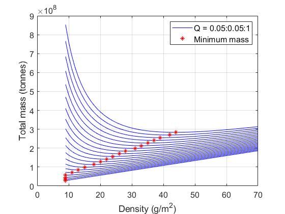
mum mass, this dependency was studied obtaining the graph in figure 3.1.
24CHAPTER 3. RESULTS 25
Figure 3.1: Variation of the total mass of the system with the areal density, for
a certain set of values of the reflectivity parameter Q. Q has a value of 0.05 for
the bottom line and 1 for the one located at the top of the graph.
Figure 3.1 shows the variation of the mass with the density and the reflec-
tivity. In the graph it is also possible to find star points that show the lowest
mass achievable for each reflectivity. It can be seen that depending on the value
of the reflectivity, the density of the spacecraft for the minimum mass changes.
For reflectivities between 0.05 and 0.2 the minimum mass corresponds with
the minimum density, whereas for reflectivities higher the minimum mass is
located in higher values for the density.
This takes place because the density affects the total mass in two differ-
ent ways: directly by itself and indirectly through the area by changing the
equilibrium point position. But this equilibrium point position also changes
with the reflectivity. The total mass is proportional to the density and the area.
So that, when the density increases, the mass tends to behave the same way
but the area decreases, creating the opposite effect and decreasing the mass.
As the reflectivity increases, the equilibrium point moves towards the Sun, in-
creasing the area needed. For reflectivities smaller than 0.2 the most important
factor when looking for the minimum mass is the direct effect of the density26 CHAPTER 3. RESULTS
and accordingly, the minimum mass point is located in the minimum density.
When the reflectivity reaches 0.2 and the equilibrium point moves closer to the
Sun, the area becomes more important when looking for the minimum mass.
This forces the minimum mass point to move to higher densities, in order to
move the equilibrium point closer to the Earth and therefore decrease the area
needed.
Based on these results, the minimum mass is obtained by choosing the min-
imum areal density and the minimum reflectivity, giving a final mass of 28.5
million tonnes. However, there is something else that needs to be kept in mind
and that is the performance of the solar sail. This performance is represented
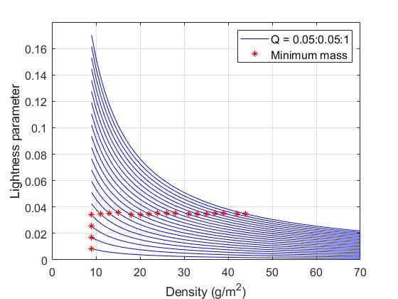
by the lightness parameter (β), whose values can be seen for each one of the
minimum mass points in Figure 3.2. The higher the value of β, the solar sail
is able to generate a greater acceleration and thus has a better performance.
Consequently, the combination that results in the minimum mass corresponds
as well with the worst performance of the sail.
It can be noted that the lightness parameter corresponding with the mini-
mum mass points increases with Q, until it stabilizes at a value of 0.035 from
Q ∼ 0.2 on. In view of these values, if a combination different from the one
resulting in the minimum mass is to be considered in order to achieve a better
sail performance, it would be reasonable to choose the first point with a light-
ness parameter of 0.035, since it is the one with the lowest mass inside this
group. As a result, two options were under study for the definition of the fi-
nal characteristics of the solar sail. The first corresponding with the minimum
mass overall and the second being the one that, inside the group of minimum
mass points for each reflectivity, has a lowest mass and a lightness parameter
of 0.035. The definition of both points can be found in table 3.1.
Table 3.1: Options considered for the spacecraft definition.
Case 1 Case 2
−2
Density (g m ) 9 9
Reflectivity 0.05 0.2
Lightness parameter (β) 0.0085 0.035
Total mass (kg) 2.85 × 10¹⁰ 5.66 × 10¹⁰
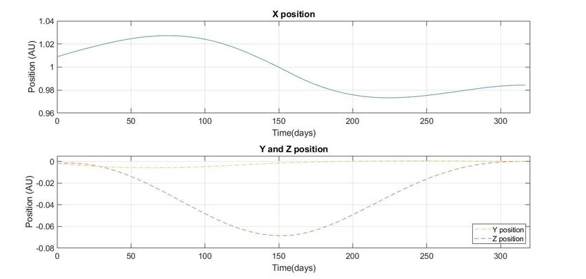
Escape trajectory time (days) 1 792 582
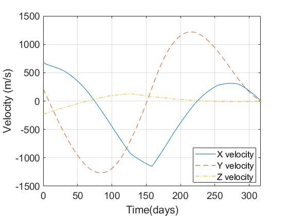
Trajectory to L1 time (days) - 317You can also read