FIXED INCOME - PARAMETERS METHODOLOGIES USED IN MARGIN CALCULATIONS

FIXED INCOME -
PARAMETERS
METHODOLOGIES
USED IN MARGIN
CALCULATIONS
MANUAL

Version 2.0 as of april 2021

1

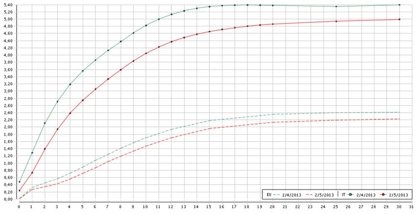
TABLE OF CONTENTS
FOREWORD ....................................................................................................... 3

EXECUTIVE SUMMARY ...................................................................................... 5

 DESCRIPTION OF THE METHODOLOGY ......................................................... 8

 1.1 Peculiarities of Fixed Income Securities .................................................. 9
 1.1.1 The pull to par phenomenon ................................................................... 9

 1.1.2 The roll down phenomenon .................................................................... 9

 METHODOLOGIES FOR DETERMINING MARGING PARAMETERS .................. 11
 2.1 Government Bonds ................................................................................ 12

 2.1.1 Main parameters .................................................................................. 12

 2.1.2 Margin Interval Calculation .................................................................... 12

 2.1.3 Defining Coverage Level........................................................................ 13

 2.1.4 Determining Proposed Margin Interval for each vertex of the curve ............ 14

 2.1.5 Defining the Duration Classes ................................................................ 15

 2.1.6 Determining the Margin Interval for Each Duration Class ........................... 17

 2.1.7 Determining the Intra-Class Offset Factor COFk ....................................... 18

 2.1.8 Determining the Inter–Class Offset Factor XOFh,k .................................... 19
 2.1.9 Priorities in Applying the Inter–Class Offset Factors XOFh,k ....................... 19

 2.2 Corporate Bonds .................................................................................... 23

 2.2.1 Classes specifications ........................................................................... 23
 2.2.2 Intra–Class and Inter-Class Offset Factors ............................................... 23

 2.2.3 Procedures for Margin Parameters Review ............................................... 24

2

FOREWORD

 3

FOREWORD

This document describes the methodology used to determine the parameters used for
Initial Margin Calculation for cash and repo contracts on government bonds and for cash
contracts on corporate bonds traded on markets where CC&G is about to intervene as
Central Counterparty.

The document is preceded by an executive summary followed by a detailed description of
the methodology, containing the underlying assumptions and the applicative details. The
document ends with a description of the margin parameters update and modification
procedure.

4|

EXECUTIVE
 SUMMARY

EXECUTIVE SUMMARY

The document describes the methodology from a conceptual standpoint beginning with
the intrinsic characteristics of bonds which do not allow the determination of margin
parameters directly from historical price series of traded bonds, as it is to the contrary
possible with equities. This description is then followed by an overview on the various
methodologies (so-called “cashflow mappings”) that may be used to associate bond price
fluctuations with variations of easily manageable risk factors, such as rates along the
zero coupon curve.

Then a description is provided about the zero coupon curve splitting into several
Vertices1. For each Vertex a Margin Interval is determined in the usual manner, that is a
value such to comprise at least a predetermined percentage (99.80%) of the actual two-
day yield fluctuations. Once the Margin Interval in Terms of Yield has been determined,
the application of the formulas linking price, yield and duration, allows to determine a
Margin Interval in Terms of Percentage Bond Price Variation.

In order to identify the Duration Classes, it is necessary to examine correlations between
zero coupon bond prices on the 45 Vertices along the curve. Paragraph 2-1-4 shows how
yield time series can be converted in bond price time series.

Once the above mentioned operations have been achieved, it is possible to build up
Duration Classes. As shown in paragraph 2-1-5, duration classes are defined as sets of
Vertices whose reciprocal correlations (identified by an index, denominated “D/U” or “div-
undiv”) are above a predetermined level (generally 0.80). It must be mentioned that this
approach may be followed in the central part of the curve, whereas in the “peripheral”
parts, a case-by-case approach must be followed.

Once duration classes have been defined, Offset Factors may be defined for positions of
opposite sign belonging to the same Duration Class (Intra–Class Offset Factor) or to
different duration Classes (Inter–Class Offset Factor).

Paragraphs 2-1-7 and 2-1-8 describe the conservative approach used to define the Intra–
and Inter–Class Offset Factors; the latter being applied according to a priority sorting
criterion .

In further detail, the Intra–Class Offset Factor is set equal to the lowest correlation
registered between Vertices comprised in the Class. Correspondingly, the Inter–Class
Offset Factor is set equal to the lowest correlation registered between the two Classes.
Regarding the priority sorting, it has been decided to follow a conservative criterion.
Therefore the low correlations registered in the short term part of the curve are applied
first and only afterwards the higher correlations registered in the medium-long term part
of the curve.

All others parameters having been determined, paragraph 2-1-9 shows how the Margin
Interval is determined for each duration Class. For this purpose the Margin Interval in
terms of Percentage Bond Price Variations determined for each Vertex, are considered.

1We have 41 vertices for the italian Government bond curve and 45 vertices for the Euro ZCB
curve.

6|

EXECUTIVE SUMMARY

The Margin Interval for each duration Class is set equal to the highest Margin Interval in
Terms of Percentage Bond Price Variations for each Vertex comprised in the Duration
Class.

7|

DESCRIPTION
 OF THE
METHODOLOGY

DESCRIPTION OF THE METHODOLOGY

1.1 Peculiarities of Fixed Income Securities
In order to determine the largest price variation for a fixed income security, its main
peculiarities must be recalled.

1.1.1 The pull to par phenomenon

Whereas the price of an equity instrument may be assumed to follow a random walk and
therefore it is not possible to determine a priori which will be the price of a given stock at
a given future date, the price of a bond converges to the parity at maturity (so–called
“pull to par phenomenon”).

1.1.2 The roll down phenomenon

The volatility of a stock is a function of the square root 2 of the time interval on which it is
measured, that volatility over a time horizon of n days is equal to n times the one-day
volatility: = √ 1 To the opposite the volatility of a bond converges to zero as the
time to maturity decreases (so–called “roll down phenomenon”).
The above mentioned phenomena preclude the recourse to analysis of price variations of
the bond itself since the price variation patterns of a bond having a certain time to
maturity τ is completely unrelated to the price variation patterns of the same bond at a
different point in time in which its time to maturity was τ +t.

2
 The apparently anti-intuitive relation linking volatility to the square root of time derives
 P 
 ln  t + 2 
 
 from the following considerations: The two-day return of a security is equal to:  Pt ,
 which, using the properties of logarithms may be written as:
 P  P  P 
 ln  t + 2  = ln  t + 2
  P
  + ln  t +1 
   P 
  Pt   t +1   t  . That is the two-day return is the sum of the two one-day
  t+2
 returns. The two-day standard deviation is equal to:
  t+2 =  2
 t +1 +  + 2 t + 2  t +1  t + 2 ,t +1
 t
 2

 . Under the assumption that returns follow a random
 walk, the correlation term ρt+2,t+1 is equal to zero. If moreover it is assumed that returns
 are identically distributed across time (independent and identically distributed returns),

  t +1 =  t  t + 2 =  t2+1 +  t2 = 2 t
 then and therefore .

9|

DESCRIPTION OF THE METHODOLOGY

 a) Cashflow Mappings Methodology

In order to measure the risk of a bond is therefore necessary to use analytical
instruments that may indicate the functional relationships of the bond price with the risk
factors to which it is exposed; such task may be fulfilled by mapping the cashflows
produced by the bond.

The simplest and most immediate type of mapping is the principal mapping, in which the
bond risk is associated with the time to maturity of its principal payment only, without
considering any other information regarding the other characteristics of the bond, in
other words, not taking into consideration the coupons paid by the bond during its life. A
more advanced type of mapping is the duration mapping, in which the risk is associated
with the bond duration3, a quantity that allows bond with coupons to transform into an
equipollent zero–coupon bond, allowing thus the comparison between bonds with
different coupon rates and between bonds with coupon and zeroes.

It is worth mentioning that both principal mapping and duration mapping identify a single
risk factor for each bond, respectively equal to the zero–coupon yield for maturity equal
to the time to maturity of the bond and to the zero–coupon yield for maturity equal to
the bond duration. Both methodologies consider as fungible the cash flows originated by
the same bond at different points in time and do not consider, within the same bond, the
imperfect correlation of yields along the curve.

A more advanced type of mapping, the so-called “cashflow mapping” allows to keep into
account also the decorrelation along the zero–coupon curve, as it takes into
consideration the risk of each single future cash flow produced by the bond, discounted
at the proper rate.

The margin parameters calculation methodology adopted by CC&G is based on Duration
mapping for non indexed Italian government bonds and on Principal mapping for other
government bonds and corporate bonds.

3 The duration D is equal to the weighted average of the maturities ti of the various cash
flows CFi, using as weights the present values (discounted at rate y) of the amounts due; k is the
 CF i (1 + y ) i t i
 n −t
 1
number of coupon per year. D =
 k
  CF i (1 + y )
 − ti
 .
 i =1

10 |

METHODOLOGIES
FOR DETERMINING
 MARGING
 PARAMETERS

METHODOLOGIES FOR DETERMINING MARGING PARAMETERS

2.1 Government Bonds
This section describes the methodology used to determine the parameters adopted in the
Initial Margin calculation for cash and repo contracts on government.

2.1.1 Main parameters

The following paragraphs aim at describing the below parameters:

 1. Bracket and number of duration classes
 2. Margin Intervals for each class (Government Bonds)
 3. Intra-Class Offset Factor (COFk)
 4. Inter–Class Offset Factor (XOFh,k)
 5. Margin Interval for Corporate Bonds
 6. Intra–Class Offset Factor for corporate bond

2.1.2 Margin Interval Calculation

In order to evaluate with the highest accuracy the possible variations of risk factors,
CC&G has divided the Italian sovereign zero–coupon curve in 41 Vertices4 xi, ranging
from 3 months to 30 years, and the Euro zero–coupon curve in 45 Vertices xi, ranging
from TN to 30 years as shown in Figure 1

4Obtained by linear interpolation from the original 25 vertices, in order to make a homogeneous
comparison with Euro zcb curve.

12 |

METHODOLOGIES FOR DETERMINING MARGING PARAMETERS

FIGURE 1: ITALIAN GOVERNMENT ZCB YIELD CURVE AND EURO ZCB YIELD
CURVE

For each Vertex xi (both for Euro and sovereign zero-coupon curve) the yield variations
for different holding periods are calculated and for each scenario (one, two or three days
fluctuations) the Margin Interval in Terms of Yield is determined 5 and set equal to such a
value as to supply a fixed Coverage Level (see next paragraph) compared to the whole
set of n-days yield variations Δy = yt+n - yt actually observed on various time horizons.

The coverage level has been fixed to give more weight to the most recent fluctuations
with respect to the older ones.

2.1.3 Defining Coverage Level

Level of coverage and, consequentially, Margin Intervals are defined by applying the
“Sovereign Risk Framework” (SRF) that basically consists in:

 ➢ a “Predictive Model”, based on dynamic market indicators, to detect early
 warnings of the progressive deterioration of Sovereign creditworthiness

 ➢ a “Toolbox” structured in order to gradually build the CCP level of protection
 against Sovereign Risk

5Calculating also the first four moments of the yield variation distribution (average, standard
deviation, skewness and kurtosis).

13 |

METHODOLOGIES FOR DETERMINING MARGING PARAMETERS

For each Band/Riskiness Level, the SRF foresees the application of the following
“Toolbox” that includes different coverage levels for one, two, three, four and five days
yield variations of the vertices of the Specific Sovereign Curve since the introduction of
the Euro (January 2nd, 1999). Conservatively the comparison with the European zero
coupon bond curve is also taken into account, whenever applicable.

Generally, the coverage levels applied to longer time brackets are lower than those
applied to shorter ones in order to limit the impact on margin levels of price variations
occurred in a distant past.

2.1.4 Determining Proposed Margin Interval for each vertex of
the curve

After defining the appropriate coverage level as from the “toolbox” in table 2-1, the
methodology adopted leads to the identification of a Margin Interval for each vertex,
according the following steps:

 1) Identification, for each vertex of the curve (both for government and euro curve),
 of the corresponding Margin Interval for each time bracket (separately for each
 holding period considered)6;

 2) Determination, for each vertex of the curve (both for government and euro zcb
 curve), of the Proposed Margin Interval (in terms of yield) as the highest Margin
 Interval of each time bracket (separately for each holding period);

 3) Determination, for each vertex of the curve (both for government and euro curve)
 separately for each holding period, of the proposed Margin Interval in terms of price
 by multiplying the Margin Interval in terms of yield times the Modified Duration;

 4) Determination, for each vertex of the curve (both for government and euro curve)
 of the Proposed Margin Interval (in terms of price) as the highest Proposed Margin
 Interval in all the holding periods considered in the analysis;

 5) Determination, for each vertex of the curve, of the Proposed Margin Interval (in
 terms of price) as the highest amount between the Proposed Margin Interval
 calculated on Euro Zcb curve and on the Sovereign Zcb curve;

 6) The Proposed Mathematic Margin Interval for the “special” Class of BTPi is equal to

6 At this step, Magin interval is defined as the average value between the first observation to be
included and the first observation to be excluded.

14 |

METHODOLOGIES FOR DETERMINING MARGING PARAMETERS

 the highest Margin Interval among all BTPi;

 7) The Proposed Mathematic Margin Interval for the “special” Class of CCTs is equal to
 the highest Margin Interval among all CCTs7;

2.1.5 Defining the Duration Classes

The brackets and the number of “ordinary” Classes are defined in order to maximize the
correlations among all the vertices in the Classes, except for inflation linked bonds (BTPi)
and for Floating Rate Bonds (CCT) that, regardless of their Duration, are instead
allocated in a “specific” Class (respectively Class XII and XIII).

In order to determine the correlations between price variations of the zero–coupon bonds
for each vertex xi along the curve yield figures are converted into price figures 8 .

For each pair of vertices xi, xj CC&G determines the complement to the ratio (so-called
"div-undiv" or "D/U") between the "diversified VaR" and the "non-diversified VaR" for
positions of opposite sign. In other words, the D/U measures the actual benefit in terms
of risk reduction arising from positions of opposite sign (and same countervalue) on
different vertices, deducted the lack of correlation between the two Vertices.

The diversified VaR is equal to the portfolio standard deviation =
√ 2 2 + 2 2 ∓ 2 comprising instruments a and b with relative weightings
respectively equal to Wa and Wb and having a correlation ρab. Assuming the relative
weights equal to 1 and –1 (positions of opposite sign) the result is:

 = √ 2 + 2 − 2 

The Undiversified VaR is equal to the portfolio standard deviation σp calculated assuming
a perfect correlation, that is ρab=1; in case of relative weights equal to 1 and –1
(therefore ρab-1) the result is: = √ 2 + 2 + = √( + )2 = | + |.

The actual diversification benefit between positions of opposite sign is assumed equal to:

 √ 2 + 2 − 2 
 − = 1 − =1−
 | + |

7 The only lookback period applied to CCTs is 18 months.
 1
8 For money market maturities, zero–coupon prices are obtained using the formula: = ,
 (1+yt )n
where n is the number of years to maturity; for maturities greater than one year the continuously
compounding is used = n .

15 |

METHODOLOGIES FOR DETERMINING MARGING PARAMETERS

Duration Classes shall comprise high correlated Vertices, generally those Vertices whose
“div-undiv” are above 0,80. In other words, Classes will be the set of Vertices whose
reciprocal “div-undiv” are generally higher than or equal to 0,80

 = { | ∈ , − ( ) ≥ Φ; ∀ , ∈ }

Whereas C is the zero–coupon curve, x a generic Vertex, Ck is the generic Duration Class
and Φ is approximately near to 0,80.

Conservatively the comparison with the correlations of the European blended curve is
also taken into account, whenever applicable.

TABLE 2.1. DIV-UNDIV- EXAMPLE 1

Table 2.1 shows how the div-undiv, for maturities comprised between 3 years and six
months and 4 years and 9 months, are generally near to 0,80, as well as for maturities
comprised between 5 years and 7 years.

16 |

METHODOLOGIES FOR DETERMINING MARGING PARAMETERS

In the “peripheral” parts of the curve - in particular in the short term part (see Table 2.2)
where jumps are more frequent given the higher sensitivity to monetary policy decisions
- a case-by-case evaluation9 is required.

TABLE 2.2. DIV-UNDIV- EXAMPLE 2

2.1.6 Determining the Margin Interval for Each Duration Class

The Proposed Mathematic Margin Interval for each Duration Class is set – as shown in
Table 2.3 – as the largest Margin Interval in Terms of Price of all the Vertices comprised
in the Class, rounded – where advisable – to the 0,05% above. The Proposed Mathematic

9
 It must be also mentioned that breaking up the zero–coupon curve in too many Classes is not desirable.
Experience has shown insofar that the number of Classes is best being kept between 10 and 15.

17 |

METHODOLOGIES FOR DETERMINING MARGING PARAMETERS

Margin Interval for the Class XII (BTPi) and XIII (CCT) is equal to the highest Margin
Interval among all the specific instruments.

In order to mitigate procyclicality, CC&G applies the required 25% buffer, only to those
instruments whose time series are shorter than 10 years.

TABLE 2.3. DETERMINATION OF THE PROPOSED MARGIN INTERVAL FOR EACH
CLASS – EXAMPLE

Applied Margin Interval is the Margin Interval in force at the date of the calculation
(which is the result of previous margin calculations and of parameters change).

A back test is performed daily on the actual price variations of the bonds included in the
margins procedure, in order to verify the ex post performance of the risk parameter
settings compared to the observed market data.

In particular, the back test compares the price variation of each bond with the Margin
Interval applied to the Class in which the Bond is included and, in case the price variation
results higher than the Margin Interval, a breach is counted.

The coverage level obtained in the back test is then calculated in order to verify the
adequacy of the Margin Interval calculated on the analysis of the volatility on the vertices
of the Italian zero coupon bond curve (for further details concerning margin parameters
review see paragraph 2.2.3).

2.1.7 Determining the Intra-Class Offset Factor COFk

In order to take into account correlation between long and short positions of bonds within
the same class of duration, offset factors are applied to reduce positions.

18 |

METHODOLOGIES FOR DETERMINING MARGING PARAMETERS

Once Duration Classes have been determined according to the aforesaid procedure, for
each Class Ck the Intra–Class Offset Factor COFk is determined.

As a general rule, COFk is equal to the smallest div-undiv between pairs of Vertices
comprised in the Class:

 = { | ∈ , min ⌊ − ( )⌋ ; ∀ , ∈ }

Prudentially COFk is rounded to the lower 5% (e. g.: 0,68 is rounded to 0,65).

Typically COFk will be found at the extreme of the secondary diagonal where the div-
undiv between the two farthest Vertices in the Class is calculated, as it can be seen in
Table 2.2.

2.1.8 Determining the Inter–Class Offset Factor XOFh,k

In order to take into account correlation between long and short positions of bonds
included in the different classes of duration (highly correlated positions), offset factors
are applied to reduce positions.

The Inter–Class Offset Factor XOFh,k between two classes Ch and Ck is determined
according to the same criterion. It is assumed equal to the lowest div-undiv between
Vertices belonging to two separate Classes. Only those Classes whose lowest div-undiv is
higher of a threshold value Ψ are eligible for Inter–Class Offsetting.

 ℎ, =
{ ℎ | ℎ ∈ ℎ , | ∈ , [ − ( )] ≥ Ψ, ∀ ∈ , ∀ ∈ , ℎ ∩ = ∅; [ −
 ( )]}

Table 2.1 provides an example of how XOFh,k is determined between two Duration
Classes. In the central part of the zero–coupon curve Ψ is approximately set at 0,35-
0,40, also with the aim of keeping the priority matrix reasonably manageable.

Once more, in the “peripheral” parts of the curve, in particular in the short term part (see
Table 2.2 ) Ψ must be necessarily evaluated on a case-by-case basis.

Experience has shown insofar that the number of XOFh,k is better kept below 30, in order
to ensure a more efficient operational management of margin parameters.

2.1.9 Priorities in Applying the Inter–Class Offset Factors
XOFh,k

The correlation between Vertices – and therefore between Duration Classes – grows with
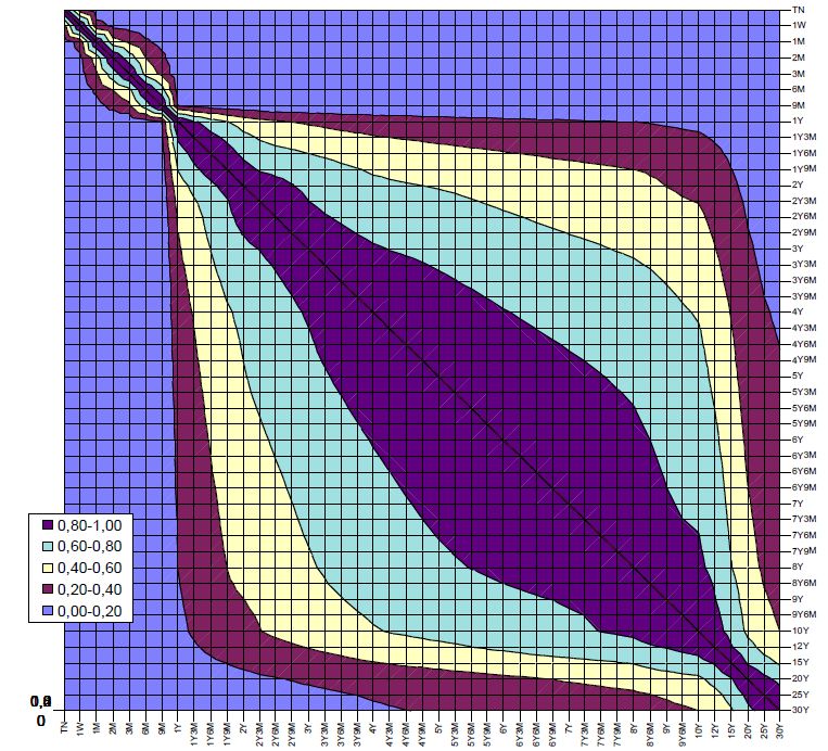
the time to maturity, as shown in Figure 2 (1 year figures). Prudentially the first XOFh,k’s

19 |

METHODOLOGIES FOR DETERMINING MARGING PARAMETERS

applied are the smallest ones measured between the low Duration Classes and only
subsequently the higher XOFh,k’s between higher Duration Classes are applied

20 |

METHODOLOGIES FOR DETERMINING MARGING PARAMETERS

FIGURE 2. CORRELATION AMONG ALL PAIRS OF VERTICES -EXAMPLE

21 |

METHODOLOGIES FOR DETERMINING MARGING PARAMETERS

FIGURE 3: PRIORITY AND INTRA / INTER CLASS OFFSET – EXAMPLE

 Class I II III IV V VI VII VIII IX X XI XII XIII
 I 5%
 Priority 1
 II 35% 20%
 Priority 2 14
 III 20% 50% 40%
 Priority 14 3 15
 IV 40% 75% 35% 25%
 Priority 15 4 16 17
 V 35% 65% 40% 25%
 Priority 16 5 18 19
 VI 25% 40% 70% 50% 35% 25%
 Priority 17 18 6 20 21 22
 VII 25% 50% 75% 55% 40% 25%
 Priority 19 20 7 23 24 25
 VIII 35% 55% 75% 55% 40%
 Priority 21 23 8 26 27
 IX 25% 40% 55% 75% 55% 25%
 Priority 22 24 26 9 28 29
 X 25% 40% 55% 70% 35%
 Priority 25 27 28 10 30
 XI 25% 35% 55%
 Priority 29 30 11
 XII 15%
 Priority 12
 XIII 10%
 Priority 13

22 |

METHODOLOGIES FOR DETERMINING MARGING PARAMETERS

2.2 Corporate Bonds

2.2.1 Classes specifications

To distinguish between the margin parameters applied to government bonds and the
margin parameters applied to corporate Bonds, a different set of classes has been
implemented.

Due to the reduced liquidity of corporate bonds, a less granular classes structure has
been adopted for these instruments.

Therefore, 5 classes have been identified taking into consideration the maturities on the
medium and long term (3,5,7,10 and 10 years +).

2.2.2 Intra–Class and Inter-Class Offset Factors

Corporate bonds price takes in account the risk free rates shape and the single issuer
financial condition, considering the specific pay-off for each corporate bond. As a
consequence, is not possible a priori to determine a correlation between the corporate
bonds prices fluctuations related to the corporate bonds Classes.

In order to take into account of the part related to the ZCB curve shape, an Intra-Class
Offset Factor (conservatively set at maximum value equal to the lower value calculated
for ZCB curve) may be applied to each corporate bonds class, subject to Internal Risk
Committee approval. No Inter-Class Offset Factor is applied.

Figure 4 provides an example of Duration Classes and corresponding Margin Intervals
separately for government bonds and corporate bonds.

23 |

METHODOLOGIES FOR DETERMINING MARGING PARAMETERS

FIGURE 4: DURATION CLASSES AND MARGIN INTERVALS – EXAMPLE

Government bonds

Corporate bonds

2.2.3 Procedures for Margin Parameters Review

Margin parameters are monitored and - if necessary - modified, basing on the periodic
back test results and, in general, on the market conditions and volatility trends.
Parameters for Italian government bonds shall be agreed with LCH.Clearnet SA before
entering into force.

24 |

CONTACT

Cassa di Compensazione e Garanzia S.p.A.

Risk Management

ccg-rm.group@euronext.com

www.ccg.it

Disclaimer

This publication is for information purposes only and is not a recommendation to engage in investment
activities. This publication is provided “as is” without representation or warranty of any kind. Whilst all
reasonable care has been taken to ensure the accuracy of the content, CC&G does not guarantee its accuracy
or completeness. CC&G will not be held liable for any loss or damages of any nature ensuing from using,
trusting or acting on information provided. No information set out or referred to in this publication shall form
the basis of any contract. The creation of rights and obligations in respect of services provided by CC&G shall
depend solely on the applicable rules and /or contractual provisions of CC&G. All proprietary rights and interest
in or connected with this publication shall vest in CC&G. No part of it may be redistributed or reproduced in any
form without the prior written permission of CC&G. CC&G disclaims any duty to update this information.
Unauthorised use of the trademarks and intellectual properties owned by the Company or other Companies
belonging to Euronext Group is strictly prohibited and may violate trademark, copyright or other applicable
laws.

© 2021, CC&G - All rights reserved

www.ccg.it