From numerical modelling - Course Introduction to data assimilation - Cerea
←
→
Page content transcription
If your browser does not render page correctly, please read the page content below

Sorbonne Université
                                 Université Paris-Saclay
      Master 2 Sciences de l'Océan, de l'Atmosphère et du Climat (SOAC)
Parcours Météorologie, Océanographie, Climat et Ingénierie pour les Observations Spatiales
                                       (MOCIS)
  Master 2 Water, Air, Pollution and Energy at local and regional scales (WAPE)

                                   Année 2018-2019

               Course Introduction to data assimilation

            From numerical modelling
               to data assimilation
                                  Olivier Talagrand

                                   8 January 2019

- What is assimilation ?

      - Numerical       weather      prediction.   Principles   and
        performances

      - Definition of initial conditions

- Bayesian Estimation

- One first step towards assimilation : ‘Optimal Interpolation’

- The temporal dimension : Kalman Filter and Variational
  Assimilation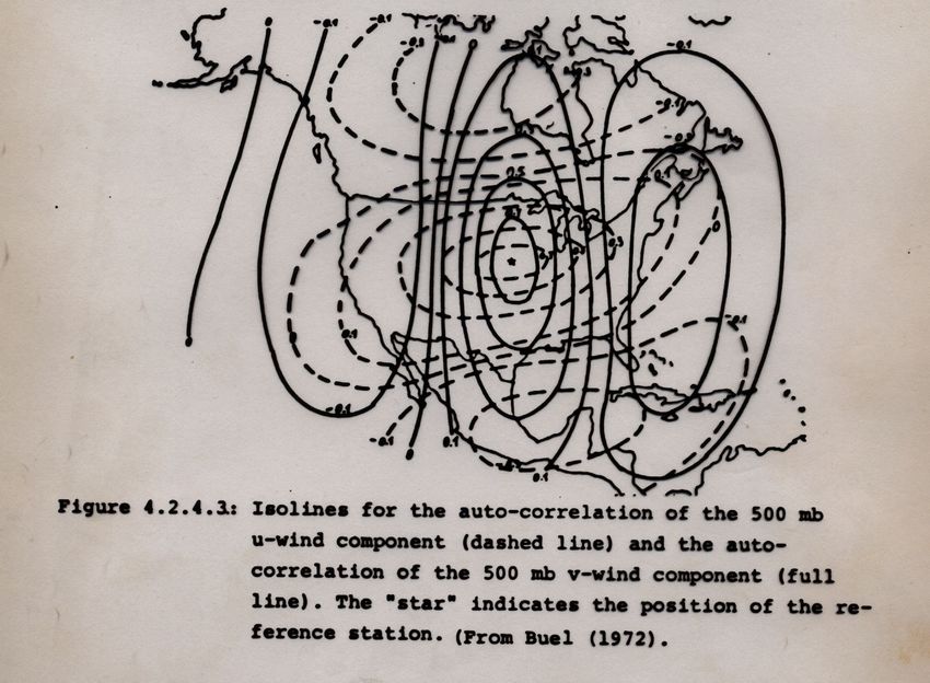
ECMWF, Technical Report 499, 2006
Pourquoi les météorologistes ont-ils tant de peine à prédire le temps
      avec quelque certitude ? Pourquoi les chutes de pluie, les tempêtes
      elles-mêmes nous semblent-elles arriver au hasard, de sorte que bien
      des gens trouvent tout naturel de prier pour avoir la pluie ou le beau
      temps, alors qu’ils jugeraient ridicule de demander une éclipse par
      une prière ? Nous voyons que les grandes perturbations se produisent
      généralement dans les régions où l’atmosphère est en équilibre
      instable. Les météorologistes voient bien que cet équilibre est instable,
      qu’un cyclone va naître quelque part ; mais où, ils sont hors d’état de
      le dire ; un dixième de degré en plus ou en moins en un point
      quelconque, le cyclone éclate ici et non pas là, et il étend ses ravages
      sur des contrées qu’il aurait épargnées. Si on avait connu ce dixième
      de degré, on aurait pu le savoir d’avance, mais les observations
      n’étaient ni assez serrées, ni assez précises, et c’est pour cela que tout
      semble dû à l’intervention du hasard.


      H. Poincaré, Science et Méthode, Paris, 1908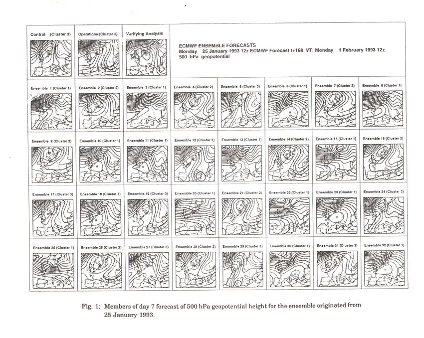
Why have meteorologists such difficulties in predicting the
    weather with any certainty ? Why is it that showers and even
    storms seem to come by chance, so that many people think it
    is quite natural to pray for them, though they would consider
    it ridiculous to ask for an eclipse by prayer ? […] a tenth of a
    degree more or less at any given point, and the cyclone will
    burst here and not there, and extend its ravages over districts
    that it would otherwise have spared. If they had been aware of
    this tenth of a degree, they could have known it beforehand,
    but the observations were neither sufficiently comprehensive
    nor sufficiently precise, and that is the reason why it all seems
    due to the intervention of chance.


    H. Poincaré, Science et Méthode, Paris, 1908


    (translated Dover Publ., 1952)

                                                                   6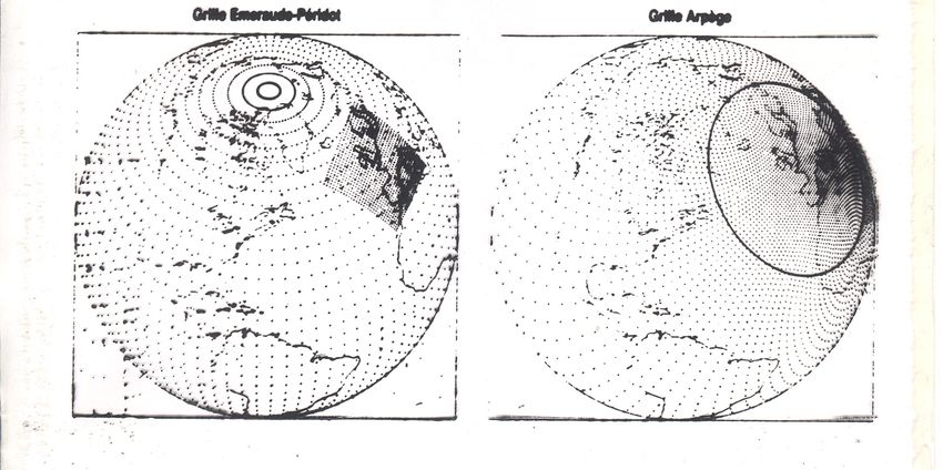
ECMWF

Satellite ADM-Aeolus has recently been launched (August 22
  2018). It carries a Lidar-Doppler instrument, called Aladin
  (Atmospheric LAser Doppler Instrument), that will measure
  the wind in the volume of the atmosphere.
Synoptic observations (ground observations, radiosonde observations),
performed simultaneously, by international agreement, in all meteorological
stations around the world (00:00, 06:00, 12:00, 18:00 UTC), and are in practice
concentrated over continents.
Asynoptic observations (satellites, aircraft), performed more or less
continuously in time.
Direct observations (temperature, pressure, horizontal components of the wind,
moisture), which are local and bear on the variables used for for describing the
flow in numerical models.
Indirect observations (radiometric observations, …), which bear on some more
or less complex combination (most often, a one-dimensional spatial integral)
of variables used for for describing the flow
y = H(x)
H : observation operator (for instance, radiative transfer equation)S. Louvel, Doctoral Dissertation, 1999
17
E. Rémy, Doctoral Dissertation, 1999
Physical laws governing the flow
Conservation of mass
Dρ/Dt + ρ divU = 0
Conservation of energy
De/Dt - (p/ρ2) Dρ/Dt = Q
Conservation of momentum
DU/Dt + (1/ρ) gradp - g + 2 Ω ∧U = F
Equation of state
f(p, ρ, e) = 0
(for a perfect gas p/ρ = rT, e = CvT)
Conservation of mass of secondary components (water in the atmosphere, salt
in the ocean, chemical species, …)
Dq/Dt + q divU = S
These physical laws must be expressed in practice in discretized (and necessarily
imperfect) form, both in space and time ⇒ numerical model
18Parlance of the trade : Adiabatic and inviscid, and therefore thermodynamically reversible, processes (everything except Q, F and S) make up ‘dynamics’ Processes described by terms Q, F and S make up ‘physics’
All presently existing numerical models are built on
  simplified forms of the general physical laws. Global
  numerical models, used either for large-scale
  meteorological prediction or for climate simulation, are at
  present built on the so-called primitive equations. Those
  equations rely on several approximations, the most
  important of which being the hydrostatic approximation,
  which expresses balance, in the vertical direction, of the
  gravity and pressure gradient forces. This forbids explicit
  description of thermal convection, which must be
  parameterized in some appropriate way.

More and more limited-area models have been developed
 over time. They require appropriate definition of lateral
 boundary conditions (not a simple problem). Most of them
 are non-hydrostatic, and therefore allow description of
 convection.

                                                           20
There exist at present two forms of discretization
- Gridpoint discretization
- (Semi-)spectral discretization (mostly for global models,
and most often only in the horizontal direction)
Finite element discretization, which is very common in many forms of
numerical modelling, is rarely used for modelling of the atmosphere. It
is more frequently used for oceanic modelling, where it allows to take
into account the complicated geometry of coast-lines.
21Schematic of a gridpoint atmospheric model
(L. Fairhead /LMD-CNRS)
22The grids of two of the models of Météo-France (La Météorologie)
In gridpoint models, meteorological fields are defined by
   values at the nodes of the grid. Spatial and temporal
   derivatives are expressed by finite differences.

In spectral models, fields are defined by the coefficients of
   their expansion along a prescribed set of basic functions. In
   the case of global meteorological models, those basic
   functions are the spherical harmonics (eigenfunctions of
   the laplacian at the surface of the sphere).

                                                              24
Modèles (semi-)spectraux
T(µ=sin(latitude), λ=longitude) =
∑ TnmYnm (µ, λ)
0≤nLinear operations, and in particular differentiation with
respect to spatial variables, are performed in spectral
space, while nonlinear operations and ‘physical’
computations (advection by the movement, diabatic
heating and cooling, …) are performed in gridpoint
physical space. This requires constant transformations
from one space to the other, which are made possible at an
acceptable cost through the systematic use of Fast Fourier
Transforms.
For that reason, those models are called semi-spectral.
27Numerical schemes have been progressively developed and
validated for the ‘dynamics’ component of models, which
are by and large considered now to work satisfactorily
(although regular improvements are still being made).
The situation is different as concerns ‘physics’, where many
problems remain (as concerns for instance subgrid scales
parameterization, the water cycle and the associated
exchanges of energy, or the exchanges between the
atmosphere and the underlying medium). ‘Physics’ as a
whole remains the weaker point of models, and is still the
object of active research.
28Centre Européen pour les Prévisions Météorologiques à Moyen Terme (CEPMMT, Reading, GB) (European Centre for Medium-range Weather Forecasts, ECMWF) Modèle hydrostatique semi-spectral Depuis mars 2016 : Troncature triangulaire TCO1279 / O1280 (résolution horizontale ≈ 9 kilomètres) 137 niveaux dans la direction verticale (0 - 80 km) Discrétisation en éléments finis dans la direction verticale Dimension du vecteur d’état correspondant ≈ 4.109 Pas de discrétisation temporelle (schéma semi-Lagrangien semi- implicite): 450 secondes
2019
2019
Persistence = 0 ; climatology = 50 at long range

   http://old.ecmwf.int/publications/library/ecpublications/_pdf/tm/
                                                      701-800tm742.pdf
ECMWF
ECMWF
ECMWF Technical
Memorandum 831

https://
www.ecmwf.int/sites/
default/files/elibrary/
2018/18746-
evaluation-ecmwf-
forecasts-
including-2018-
upgrade.pdf
ECMWF Technical
Memorandum 831

https://
www.ecmwf.int/sites/
default/files/elibrary/
2018/18746-
evaluation-ecmwf-
forecasts-
including-2018-
upgrade.pdf
ECMWF Technical
Memorandum 831

https://
www.ecmwf.int/sites/
default/files/elibrary/
2018/18746-
evaluation-ecmwf-
forecasts-
including-2018-
upgrade.pdf
ECMWF

        Dotted curves: seasonal values
        Full curves : four-season average
ECMWF Magnusson and Källén, Mon. Wea. Rev., in press
Remaining Problems
 Mostly in the ‘physics’ of models (Q and F terms in basic
equations)
- Water cycle (evaporation, condensation, influence on radiation
absorbed or emitted by the atmosphere)
- Exchanges with ocean or continental surface (heat, water,
momentum, …)
-…

- What is assimilation ?

      - Numerical       weather      prediction.   Principles   and
        performances

      - Definition of initial conditions

- Bayesian Estimation

- One first step towards assimilation : ‘Optimal Interpolation’

- The temporal dimension : Kalman Filter and Variational
  Assimilation
Purpose of assimilation : reconstruct as accurately as possible the state of the
atmospheric or oceanic flow, using all available appropriate information. The latter
essentially consists of
The observations proper, which vary in nature, resolution and accuracy, and
are distributed more or less regularly in space and time.
The physical laws governing the evolution of the flow, available in practice in
the form of a discretized, and necessarily approximate, numerical model.
‘Asymptotic’ properties of the flow, such as, e. g., geostrophic balance of middle latitudes. Although
they basically are necessary consequences of the physical laws which govern the flow, these
properties can usefully be explicitly introduced in the assimilation process.Both observations and ‘model’ are affected with some uncertainty ⇒
uncertainty on the estimate.
For some reason, uncertainty is conveniently described by probability
distributions (don’t know too well why, but it works; see, e.g. Jaynes,
2007, Probability Theory: The Logic of Science, Cambridge University
Press).
Assimilation is a problem in bayesian estimation.
Determine the conditional probability distribution for the state of the
system, knowing everything we know (see Tarantola, A., 2005, Inverse
Problem Theory and Methods for Model Parameter Estimation, SIAM).
46Assimilation is one of many ‘inverse problems’ encountered
in many fields of science and technology
• solid Earth geophysics
• plasma physics
• ‘nondestructive’ probing
• navigation (spacecraft, aircraft, ….)
• …
Solution most often (if not always) based on Bayesian, or
probabilistic, estimation. ‘Equations’ are fundamentally the
same.Difficulties specific to assimilation of meteorological observations :
- Very large numerical dimensions (n ≈ 106-109 parameters to be
estimated, p ≈ 4.107 observations per 24-hour period). Difficulty
aggravated in Numerical Weather Prediction by the need for the forecast to
be ready in time.
- Non-trivial, actually chaotic, underlying dynamics
Relative cost of the various components of the operational prediction
suite at ECMWF (september 2015, J.-N. Thépaut) :
- 4DVAR: 9.5%
- Ensemble Data Assimilation (EDA) : 30%
EDA produces both the background error covariances for 4D-Var and
the initial perturbations (in addition to Singular Vectors) for EPS.
- High resolution deterministic model : 4.5%
- Ensemble Prediction System (EPS) : 22%
- Ensemble hindcasts : 14%
- Others : 20% (among which 17% for computation of boundary
conditions of a number of limited-area models ; those 17% include both
assimilation and forecast)
Assimilation over 24 hour of observations takes more than 40% of the
computing power devoted to 10-day operational prediction
z1 = x + ζ1
density function
p1(ζ) ∝ exp[ - (ζ2)/2s1]
z2 = x + ζ2
density function
p2(ζ) ∝ exp[ - (ζ2)/2s2]
ζ1 and ζ2 mutually independent
P(x = ξ | z1, z2) ?z1 = x + ζ1
density function
p1(ζ) ∝ exp[ - (ζ2)/2s1]
z2 = x + ζ2
density function
p2(ζ) ∝ exp[ - (ζ2)/2s2]
ζ1 and ζ2 mutually independent
P(x = ξ | z1, z2) ?
x = ξ ⇔ ζ1 = z1-ξ and ζ2 = z2 -ξ
• P(x = ξ | z1, z2) ∝ p1(z1-ξ) p2(z2 -ξ)
∝ exp[ - (ξ -xa)2/2pa]
where 1/pa = 1/s1 + 1/s2 , xa = pa (z1/s1 + z2/s2)
Conditional probability distribution of x, given z1 and z2 :N [xa, pa]
pa < (s1, s2) independent of z1 and z2Conditional expectation xa minimizes following scalar objective
function, defined on ξ-space
ξ → J(ξ) ≡ (1/2) [(z1 - ξ)2 / s1 + (z2 - ξ)2 / s2 ]
In addition
pa = 1/ J’’(xa)
Conditional probability distribution in Gaussian case
P(x = ξ | z1, z2) ∝ exp[ - (ξ -xa)2/2pa]
J(ξ) + CstEstimate
xa = pa (z1/s1 + z2/s2)
with error pa such that
1/pa = 1/s1 + 1/s2
can also be obtained, independently of any Gaussian hypothesis, as
simply corresponding to the linear combination of z1 and z2 that minimizes
the error Ε [(xa-x) 2]
Best Linear Unbiased Estimator (BLUE)z1 = x + ζ1
z2 = x + ζ2
Same as before, but ζ1 and ζ2 are now distributed according to exponential law
with parameter a, i. e.
p (ζ) ∝ exp[-|ζ |/a] ; Var(ζ) = 2a2
Conditional probability density function is now uniform over interval [z1, z2],
exponential with parameter a/2 outside that interval
E(x | z1, z2) = (z1+z2)/2
Var(x | z1, z2) = a2 (2δ3/3 + δ2 + δ +1/2) / (1 + 2δ), with δ = ⏐z1-z2⏐/(2a)
Increases from a2/2 to ∞ as δ increases from 0 to ∞. Can be larger than variance 2a2
of original errors (probability 0.08)Bayesian estimation State vector x, belonging to state space S (dimS = n), to be estimated. Data vector z, belonging to data space D (dimD = m), available. z = F(x, ζ) (1) where ζ is a random element representing the uncertainty on the data (or, more precisely, on the link between the data and the unknown state vector). For example z = Γx + ζ
Bayesian estimation (continued)


   Probability that x = ξ for given ξ ?

            x=ξ      ⇒ z = F(ξ, ζ)


   P(x = ξ | z) = P[z = F(ξ, ζ)] / ∫ξ’ P[z = F(ξ’, ζ)]


   Unambiguously defined iff, for any ζ, there is at most one x such that z = F(x, ζ).


   ⇔ data contain information, either directly or indirectly, on any component of
      x. Determinacy condition.
Bayesian estimation is however impossible in its general theoretical
form in meteorological or oceanographical practice because
• It is impossible to explicitly describe a probability distribution in a space
with dimension even as low as n ≈ 103, not to speak of the dimension n ≈
106-9 of present Numerical Weather Prediction models (‘curse of
dimensionality’).
• Probability distribution of errors on data very poorly known (model errors
in particular).One has to restrict oneself to a much more modest goal. Two
approaches exist at present
Obtain some ‘central’ estimate of the conditional probability
distribution (expectation, mode, …), plus some estimate of the
corresponding spread (standard deviations and a number of
correlations).
Produce an ensemble of estimates which are meant to sample the
conditional probability distribution (dimension N ≈ O(10-100)).Courtier and Talagrand, QJRMS, 1987
Courtier and Talagrand, QJRMS, 1987
500-hPa geopotential field as determined by : (left) operational assimilation system of
French Weather Service (3D, primitive equation) and (right) experimental variational system
(2D, vorticity equation)
Courtier and Talagrand, QJRMS, 1987
Random vector x = (x1, x2, …, xn)T = (xi) (e. g. pressure, temperature, abundance of
given chemical compound at n grid-points of a numerical model)
Expectation E(x) ≡ [E(xi)]
; centred vector x’ ≡ x - E(x)
Covariance matrix
E(x’x’T) = [E(xi’xj’)]
dimension nxn, symmetric non-negative (strictly definite positive except if linear
relationship holds between the xi’‘s with probability 1).
Two random vectors
x = (x1, x2, …, xn)T
y = (y1, y2, …, yp)T
E(x’y’T) = E(xi’yj’)
dimension nxp
Covariance matrices will be denoted
Cxx ≡ E(x’x’T)
Cxy ≡ E(x’y’T)
Random function Φ(ξ) (field of pressure, temperature, abundance of given
chemical compound, … ; ξ is now spatial and/or temporal coordinate)
Expectation E[Φ(ξ)] ;
Φ’(ξ) ≡ Φ(ξ) - E[Φ(ξ)]
Variance Var[Φ(ξ)] = E{[Φ’(ξ)]2}
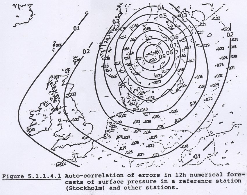
Covariance function
(ξ1, ξ2) → CΦ(ξ1, ξ2) ≡ E[Φ’(ξ1) Φ’(ξ2)]
Correlation function
Corϕ(ξ1, ξ2) ≡ E[Φ’(ξ1) Φ’(ξ2)] / {Var[Φ(ξ1)] Var[Φ(ξ2)]}1/2
•After N. Gustafsson
After N. Gustafsson
After N. Gustafsson
You can also read